
We extend the analysis we sketched in Castagna [4] and we provide an application of the framework we introduced to incrementally evaluate financial contracts within a financial institution’s balance sheet.
1 Introduction
In Castagna [4] we sketched a framework to evaluate a contract inserted within the balance sheet of a financial institution. The main result of that work is the importance to assess the impact that the contract’s insertion in the bank’s books causes in terms of changes of the value of the bank. This is tantamount to saying that a contract has a value to the bank that equals its incremental (or marginal) contribution to the total net value of the bank.
The first consequence of this approach is that the (incremental) value to the bank is a subjective quantity that does not need to be that same as the price quoted and dealt in the market. The difference between price and value of a contract is a concept that we stressed in Castagna [3] and [2]: For an evaluator that is a hedger/replicator, the price of a (derivative) contract is just the payment terms that both parties agree upon when closing the deal; the value of the same (derivative) contract is the present value of the costs paid to replicate the intermediate and final pay-off until the expiry, which in turn is the incremental change in the total hedger/replicator’s net value.
The second consequence is that the valuation should be correctly operated by considering the existing balance sheet structure. The main result from the analysis in Castagna [3] is that, if the contract is sufficiently small so that it does not alter (for practical purposes) the probability of default of the evaluator (bank), then the approximated value can be fairly considered as the equivalent to the algebraic sum of the value of i) an otherwise identical risk-free contract (the “pure” value”), ii) the Credit Value Adjustment CVA and iii) the Funding Value Adjustment FVA referring to the same contract. If the contract has a large notional so that it changes the evaluator’s default probability, then the value has to be determined in a more precise fashion by algebraically adding to the sum above the term iv) Limited Liability Value Adjustment (LLVA). The latter quantity is somehow similar to the more common Debit Value Adjustment (DVA), in that it affects the value of the contract in the opposite direction than the CVA; nonetheless it cannot be considered as equivalent to the DVA for many reasons that we thoroughly discuss in Castagna [3].
Only the value of a contract can be incremental. The concept of incremental price is meaningless, because the price cannot include all the incremental valuations referring to the parties involved in the transaction, or two generic parties that would trade in that contract if the price is only a quote not yet dealt. Clearly we are not saying here that the two parties do not consider their own incremental value when bargaining before closing the deal at the agreed price: on the contrary, they will try to push the price as near as possible to the (likely diverging) values they assign to the contract. The effectiveness of this effort depends on the relative bargaining strength existing between the two parties.
The reference system, with respect to which the bank evaluates the incremental impact of the new contract it trades, should be the economic value of the bank to its shareholders. In fact, shareholders are the last claimants on the residual value of the assets, so that the value to them clashes with the ultimate value of the bank, after having considered the payment of all the other stakeholders that have a higher grade in the claimants’ order. The only way to compute this value is to jointly evaluate all the assets and liabilities (investments, securities, contracts, etc.), taking into account the limited liability that is granted to the shareholders, to come up with the net wealth of the bank. We would like to stress the fact that if the shareholders directly, or (as it is usually the case) the bank’s management indirectly, miximise the bank’s value, they are also acting in the best interest of all other senior claimants to the assets’ value (e.g.: bond holders, depositors, etc.). The present work is a two-part article. In the current first part, we will lay out a general framework to calculate the bank’s value. The framework allows to shed some light also on the economic meaning of the Capital Value Adjustment (KVA) of a contract.
In the second part of the article, we will show how to apply the framework to the evaluation of a contract that is inserted in the existing bank’s balance sheet and how to properly compute the xVAs quantities. Finally, we will see how to conciliate the apparently theoretical unsound market practices to evaluate derivative contracts, and the nowadays standard results of the modern financial theory, namely the Modigliani-Miller (MM) theorem (see Modigliani and Miller, [9]).
The analytical details of the results presented below can be found in an extended version of this work, available at www.iasonltd.com in the research section.
2 A Continuous-Time Setting for Incremental Valuation of Financial Contracts
In order to generalise the discrete-time setting sketched in Castagna [3], we needto work in a general equilibrium framework, since it is not generally possible to determine a single equivalent probability measure based on a no-arbitrage argument that relies on a dynamic replication. We will refer to that one outlined in Cox, Ingersoll and Ross (CIR, [5]), although we relax some of its assumptions. Namely, we will work in an economy where a single good is produced by means of N production technologies whose transformation process is governed by a system of stochastic processes.
Each technology is affected by K state variables Yk (with k= {1…..K} ), whose evolution too is governed by a system of stochastic variables.
There is a single interest rate r at which a fixed number of economic agents may borrow or lend but, differently from CIR [5], we allow for the default of the borrower, which means that the terminal pay-off of a loan includes the expected losses due to the borrowers’ default. Finally, another assumption of CIR [5] we relax is that all economic agents have an identical utility function à la Neumann-Morgenstern: we consider a specific utility function for each economic agent and a general utility function that can be seen as a sort of average of the single agents’ utility functions.
The possibility to have different utility functions allows the presence of different risk-premia over the risk free rate r within the expected yield of the contingent claims possibly traded in the economy, whose pay-offs may depend on the K state variable and the wealth of a single agent, or of the entire economy aggregate wealth. The relaxing of the assumptions of the CIR [5] setting are necessary to distinguish between the fair (objective) price of a contract (contingent claim) and its (subjective) value.
Let us consider the value of the bank to shareholders at time t, VB(t): assuming that in the banks’ balance sheet there are I assets Ai(t), cash B(t) and J liabilities (debt) Lj(t), the evolution of the value of the bank can be written as:

The dynamics of all three components is stochastic. As such, the dynamics of the bank value can be described by a general SDE:

Assuming that any financial contract depend on the K risk factors and that the cash is invested at the risk-free rate r, which is a variable that depends on the stochastic factors as well, it can be shown[1] that
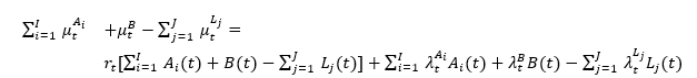
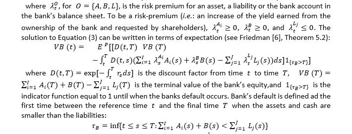
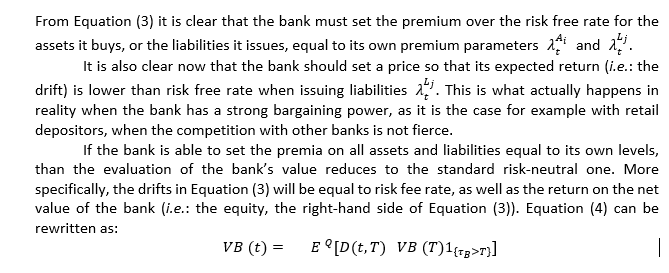
Some comments are in order: the expectation in Equation (4) is taken under the real world measure P , which means that all the drifts of the risk factors Yk are those of the real world dynamics. It should be noted that the discounting is operated with the risk free rate r as it is typically the case when the expectation is taken under the risk neutral measure Q.
i.e.: when the dynamics of the risk factors are risk neutral. To account for the error made in discounting with the risk free rate pay-offs that depend on real world dynamics of the risk factors, we add an adjustment equal to the risk-premia for all risk factors, referring to each contingent claim in the assets and in the liabilities of the bank’s balance sheet.
We have now to examine two possible cases when the banks buys an assets, or issue debt.
The Bank is Price Taker
Let us assume that the bank buys all assets in the market and it has no greater bargaining power than any other agent. In this case, the bank must accept the prices set by the market for all the assets it buys. The bank funds the purchase of the assets by issuing debt claims whose price is also set by the creditors, and it passively has to accept it since it has no bargaining power. This assumption implies that the drift of each asset is determined by the market with no possibility for the bank to affect it. The same reasoning can be applied also to debt claims in the liabilities.
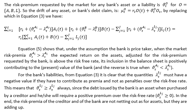
In conclusion, when the bank has to issue debt claims whose price is set by the market, it will pay twice the risk-premium: the risk-premium embedded in the price required by the buyers (creditors of the bank), and the risk-premium that the bank has not been able to include in the price. While for the assets the market’s and bank’s risk-premia are affecting the total bank value only for the net difference, for the liabilities the difference is actually a sum of two risk-premia (since they must have opposite signs) and as such acting on an aggregated basis on the bank value.
The Bank is Price Maker
Let us assume that the bank is able to set the price when buying assets and when issuing new debt. In this circumstances, the price should be such that it embed a risk-premium such that the bank value at least does not decline after the inclusion of the new asset, or new liability, in the bank’s balance sheet.
2.1 An Interpretation of the KVA
The Capital Value Adjustment (KVA) is the most recent item of the list of adjustments to the “pure” value of a contract, and it has been analysed by several authors: for an excellent review of the matter, and the regulatory and managerial concerns that originate the need for such adjustment, we refer to Prampolini and Morini [10] and the bibliography therein, which contains all the relevant literature at the time of writing.
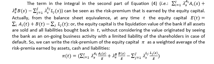
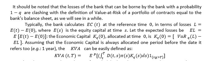
It is the adjustment in the evaluation formula (4) when the equity capital is set in such a way that it matches the Economic Capital as defined above. Some considerations are in order:
• the definition of Economic Capital given above can be applied both to risk-based measure (e.g.: simulation models applied to the bank’s balance sheet) and non-risk-based measures (e.g.: regulatory formulae): for a discussion of both types of measures, see Prampolini and Morini [10];
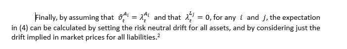
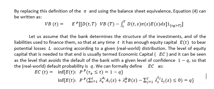
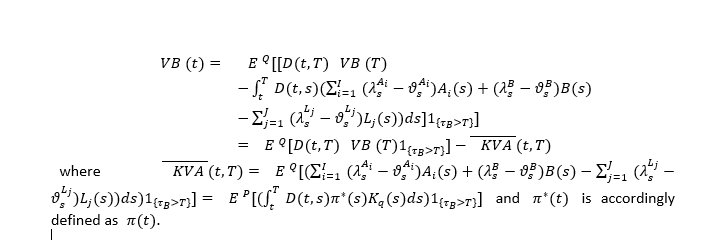
• the KVA is consistently computed only under the real-world measure P and it is discounted with the risk-free rate: these are not assumptions or choices arbitrarily made, but both are naturally derived from the framework sketched above (different discount factors can be found in Prampolini and Morini [10], Kjaer [8], Brigo et al.[1], Green et al. [7]: in some cases the discount factors include the intensity of default of the counterparty and of the bank, in any case they are not consistently derived within an equilibrium framework such as the one above). When one wants to compute the bank’s value under the risk-neutral measure, the inclusion of the KVA is not consistent, unless the adjustment includes only the difference between the bank’s and the market’s risk-premia, in which case Equation (4) becomes:
• the remuneration of the Economic Capital is given by only the risk-premia embedded in the assets, cash (bank account) and liabilities, either set by the market or by the bank depending on the bank’s bargaining power in each case. This result in in striking contrast with all the literature publicly available at the time of writing (see the point above), where the remuneration encompasses the entire return on the contracts in the balance sheet. This will produce a double counting of the risk-free rate within the calculation of the bank’s value, which will also imply a wrong adjustment if the bank is able to set a contract’s price. Our result descends from the general equilibrium framework and is valid in the case the value is computed under the real-world measure, otherwise the inclusion of the KVA adjustment is quite untenabale;
• the risk-premium of the equity capital is a weighted average of the risk-premia of the different items of the balance-sheet: when the bank has pricing power, it can require a premium proportional to the risk of the contract and the incremental Economic Capital needed to preserve the same probability of default of the bank. Pricing based on RAROC criteria are common choices, lately suggested also in Prampolini and Morini [10] and Brigo et al.[1];
The framework that we have sketched above can be used in practice to evaluate the impact of a new contract inserted in the bank’s balance sheet, or: the incremental value of the contract to the bank. We will show how to do that in the second part of the article.
References
[1] D. Brigo, M. Francischello, and A. Pallavicini. An indifference approach to the cost of capital constraints: Kva and beyond. available at arxiv.org, 2017.
[2] A. Castagna. On the dynamic replication of the DVA: Do banks hedge their debit value adjustment or their destroying value adjustment? Iason research paper. Available at http://iasonltd.com/resources.php, 2012.
[3] A. Castagna. Pricing of derivatives contracts under collateral agreements: Liquidity and funding value adjustments. Iason research paper. Available at http://iasonltd.com/resources.php, 2012.
[4] A. Castagna. Towards a theory of internal valuation and transfer pricing of products in a bank: Funding, credit risk and economic capital. Iason research paper. Available at http://www.iasonltd.com, 2013.
[5] J.C. Cox, J. E. Ingersoll, and S. A. Ross. An intertemporal general equilibrium model of asset prices. Econometrica, 53(2):363–384, 1985.
[6] A. Friedman. Stochastic Differential Equations and Applications, Volume 1. Academic Press, 1975.
[7] A. Green, C. Kenyon, and C Dennis. Kva: Capital valuation adjustment. available at arxiv.org, 2014.
[8] M. Kjaer. Kva from the beginning. available at ssrn.com, 2017.
[9] F. Modigliani and M.H. Miller. The cost of capital, corporation finance and the theory of investment. The American Economic Review, 48(3):261–297, 1958.
[10] A. Prampolini and M. Morini. Derivatives hedging, capital and leverage. available at ssrn.com, 2018.
[1] See the extended version of the paper for the complete proof.

