In the previous article [RAF15] we stressed the necessity of developing specific measures of the Operational Risk (OpRisk) for the Risk Appetite Framework (RAF) in the financial services’ industry.

Although we recommended considering a performance measure (based on a ratio of the losses over the revenues) rather than a pure risk one (based only on the losses), in this article we will focus our efforts on the estimation of the losses, considering that the revenues are usually provided by the CFO with already well developed and established models.

In particular we suggest to develop two different models: one to cover the Operational Losses (OpLosses) from the Event Types (ETs) 4 and 7, “clients, products & business practices” and “execution, delivery & process management” [BCBS04], related to the Compliance and Organizational Risks. The other one to cover the OpLosses from the ET6, “business disruption and system failures” [BCBS04], related to the Information and Communication Technology Risk (ICT Risk).

The outcomes of both models are useful to measure the OpRisk of the financial institution under examination, but the necessity of distinguishing their results arises from the nature of these OpLosses. As a matter of fact, the ICTRisk’s main effects (the indirect ones) are not usually registered in the datasets, so these models need not be based mainly on the registered losses. On the other hand the Compliance and Organizational Risks (at least in case they intersect the OpRisk, that it is their perimeter that we consider here) are well described by the data collected in the standard OpRisk datasets (considering the OpLosses from the ETs 4 and 7 respectively).

In this article we present a model of the OpLosses from the ETs 4 and 7 and, at the end, we briefly explain how to use the OpLosses’ forecasts to obtain an Operational RAF measure that considers also the related revenues and some Key Risk Indicators (KRIs). Note that, once a model considering also the indirect losses is developed, this procedure could be straightforwardly extended to the second typology of models, obviously choosing proper revenues and KRIs.

1.      The model

The idea is to model the cumulative OpLosses from the ETs 4 and 7 of a specific division of a financial institution over a fixed period of time – that goes from one month to one year.

First of all, we consider the specific characteristics of the OpLosses time series, where there is usually a standard quantity of losses per day with few huge peaks – usually clusters of out-of-range amounts in specific periods of the year, e.g., near the closure of the quarters, especially at the end of the year and at end of the 1st Semester.

We divide the cumulative OpLosses (OpL) into two components, the Body (B) and the Jump (J), that respectively represent the most common and small losses’ contribution and the extraordinary (in size) ones’ contribution. Therefore, it holds

with

We assume that the change in a quantity (ΔX for a given quantity X) is the one happening over one day (Δt >= 1).

Note that, if we consider long periods of time, the cumulative OpLosses can be approximated by continuous time stochastic processes. Therefore, regarding the Body component B, we choose to represent it as a scaled Wiener process with drift of the following type:

where µ(t) is the deterministic instantaneous mean of the Body component OpLosses at instant t and σ (assumed constant through time) is the deterministic instantaneous standard deviation of the Body component OpLosses. Finally W is a Wiener process.

Regarding the Jump component, we have to represent not only the severity of the OpLosses, but also the frequency, particularly important for our purposes. So we choose to represent the Jump component J as an inhomogeneous compound Poisson process with lognormal distribution of the following type:

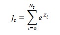
where the frequency of the jumps is described by the stochastic process N (independent from the Wiener process W), an inhomogeneous Poisson process with intensity λ(t), a given deterministic function of time.

This intensity function (λ(t)), necessary to represent the seasonality of the OpLosses, is defined by the scaled maximum of three periodic functions:

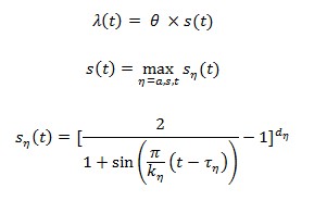
where

• θ is a positive constant representing the maximum expected number of jumps per unit of time;
• s(t) is a periodic function representing the normalized jump intensity shape;
• the parameters of s(t) are the following: the period of the function  is represented by the positive value , i.e. the jump occurrence exhibits peaking levels at multiples of  years (usually  annual,  biannual,  quarterly). The first peak of the function  is at time  in [0,k]. Finally, the positive exponent  allows us to adjust the dispersion of jumps around peaking times and to create a wider shape the lower the value is; moreover, it has a stronger effect (i.e. wider shape) the longer the period is.

Note that the form of the function  is the one used in the model of Geman and Roncoroni (see [GR06]) for representing the seasonality of the electricity prices. We choose this typology of functions because it fits also the intensity of the OpLosses’ jumps, that usually appear in short (referring to the time) clusters at the end of accounting periods.

On the other hand the severity of the Jump component J is described by the random variables , that are independent and identically distributed (iid) with normal distribution, independent from the Wiener process W and the counting process N.

Summarising we assume the OpLosses happen continuously (as a random walk) through time with sudden independent jumps lognormally distributed (as an inhomogeneous compound Poisson process with lognormal distribution). Thus the distribution of losses at the end of any finite interval of time is the sum of a normal with known mean and constant variance and (eventually) of lognormal(s).

2.      The RAF measure

The proposed model (or an equivalent one in the ICTRisk), opportunely evaluated, could be directly considered as a RAF measure (even if we do not suggest that). In fact, we could obtain an empirical distribution of the loss via a Montecarlo simulation procedure. Once the simulations from the current distribution have been performed, we obtain the forecasts (for example quarterly through the year) selecting the quantile we are interested in to represent the Profile of the bank, calling it “Position”. For example we could choose 50%, i.e. we use a VaR(50%). Moreover, at the beginning of the year, we could conventionally choose the VaR(40%) and the VaR(70%) (called “Target” and “Trigger”) to fix for the year under examination the Appetite and the Tolerance values of the division respectively.

Note that the choice of the quantiles should depend on the history and the strategic choices of the company. For example, if we are satisfied with the recent results and there are not relevant changes in the business, we can fix for the Position 50%. On the other hand, if we want to reduce risk since in the last years the business has suffered risks that we eliminated, we would choose a threshold such as 40%. On the contrary, if we have just added a product riskier than the others we offer (because of its related earnings), we would accept a 60% threshold.

In any case we think the Appetite should usually be represented by a quantile lower than the Position one and the Trigger higher because, regarding the former context, the top management usually challenges the business management to perform better and, regarding the latter context, the top management sets a warning value that, if it have been already breached, it would have triggered actions to reduce the risk at an acceptable level.

However, this framework could perform in a better way using a performance measure, rather than a pure risk one.  As a matter of fact, we think that it is better to judge the losses’ results (the “consequences” of the risks taken by the financial institution) valuating them in comparison to the ones of the revenues (the “sources” of the risks), rather than valuating them as a pure stand-alone measure.  Note that this reasoning is especially correct for the OpRisk, where the losses are strictly related to the volume of the business and so to the earnings.

So we suggest to consider a ratio of the losses over the revenues, obtaining as results new values of the Position, the Target and the Trigger (we keep the same names previously used, but now we consider the revenues as also inserted in the measure). Furthermore, we propose a couple of adjustments to the value of the losses used in the Profile of the measure (i.e. the Position).

The first correction allows us to insert a view on the actual business based on the current year’s estimated revenues, that are easier than the losses to predict (because they are less volatile) and, as said before, have a direct influence on the losses, especially in the OpRisk. Therefore, we introduce what we call “Business Adjustment”: to modify the results of the losses we could use a function of the growth rate of the revenues.

The second correction, called “Indicator Adjustment”, would insert a forward looking perspective focusing, among the others, on the emerging risks that the bank faces and will face, weighting this effect on the strategic choices of the Board/CEO. It would focus on the Compliance and the Organizational Risks (or on the ICTRisk), seen as main drivers, respectively, of the future OpLosses of the ET4 and ET7 (or of the ET6).

The main idea behind the Indicator Adjustment is to insert the “tomorrow” in the forecasts and in the actual losses used in the measure. In that case, we would choose a proper set of KRIs with two drivers in mind: they should give a forward-looking view (with an accent on the emerging risks) and they should be not too many, focusing only on the highest impact risks. Therefore, to insert the second correction we advise choosing a proper corrective capped function whose outcomes depend on the performance of the KRIs chosen.

Note that while the Business Adjustment would only apply to the Forecasts of the OpLosses, the Indicator Adjustment would apply to both the Forecasts and the Actual OpLosses.

Indeed in the former case we would be “refining” the Forecasts, whereas in the latter we would be only partially “refining” the Forecasts. In reality the main goal of the Indicator Adjustment is to highlight the effects of the risks that will happen in the future.

The reason is that the Indicator Adjustment could allow the measure to consider not only the effects that will be seen in the results of the year under examination, but also the ones that will be seen in the following few years. As a matter of fact, it is important to highlight that most of the OpLosses have a time gap, measurable in years, between the date of the Event that originates the Economic Manifestations and their booking dates.

Finally, note that the insertion of the Indicator Adjustment in the measure could also be seen as a way the Board/CEO chooses to discount (or increment) the effective OpLosses of a percentage (linked to the cap of the function) related in reality to the quantity of incentives (or disincentives) adopted by the top management to reduce the future risks that the bank will face because of the choices of the current year.

Bibliography

[BCBS04] Basel Committee on Banking Supervision, “International convergence of capital measurement and capital standards” (Basel II), Bank of International Settlements, June 2004. A revised framework comprehensive version, June 2006.

[BankIt13] Banca d’Italia, “Nuove disposizioni di vigilanza prudenziale per le banche”, Circolare n. 263, December 2006. 15th Review, July 2013, partial version.

[CS14] Credit Suisse AG, “Litigation – more risk, less return”, Ideas engine series – Equity research Europe multinational banks, June 2014.

[FSB10] Financial Stability Board, “Intensity and effectiveness of SIFI supervision”, November 2010.

[FSB13] Financial Stability Board, “Principles for an effective risk appetite framework”, November 2013.

[GR06] H. Geman and A. Roncoroni, “Understanding the fine structure of electricity prices”, Journal of Business, Vol. 79, No. 3, May 2006.

[RAF15] F. Sacchi, “Risk Appetite Framework: considerations on Operational Risk measures – Part I”, FinRiskAlert.com.

[SSG09] Senior Supervisors Group, “Risk management lessons from the global banking crisis of 2008”, October 2009.

[SSG10] Senior Supervisors Group, “Observations on developments in risk appetite frameworks and it infrastructure”, December 2010.