
Following the overview provided in [3] “IFRS17 is coming soon”, this article focuses on a potential definition of Risk Adjustment (RA) that departs from the Risk Margin one under SII and provides a methodology for its release in the Income Statement (IS). The mathematical background is accompanied by numerical examples.
Under IFRS17 the total Liabilities are given by the sum of the Liability for Incurrent Claims (LIC), a reserve meant to cover the outstanding claims, and the Liability for Remaining Coverage (LRC). The latter is defined as the sum of the technical reserves, that, in turn, is given by the Present Value of Future Cash Flows (PVFCFs) plus the Risk Adjustment (RA), and the accountant reserve named Contract Service Margin (CSM). The RA is a provision for the risk, reflecting the level of compensation the insurer demands for bearing the uncertainty embedded in the amount and timing of CFs related to non-financial risks, excluding the operational one, as not directly generated by insurance contracts. The International Accounting Standard Board (IASB) has prescribed the need for the undertakings to disclose the confidence level chosen for the calculation, to show their degree of risk aversion, but has not specified a technique for the RA derivation, rather providing general characteristics it shall respect.
[B91] …the RA for non-financial risk shall have the following characteristics:
- risks with low frequency and high severity will result in higher RA for non-financial risk than risks with high frequency and low severity
- for similar risks, contracts with a longer duration will result in higher RA for non-financial risk than contracts with a shorter duration
- risks with a wider probability distribution will result in higher Risk Adjustments for non-financial risk than risks with a narrower distribution
- the less that is known about the current estimate and its trend, the higher will be the Risk Adjustment for non-financial risk
- to the extent that emerging experience reduces uncertainty about the amount and timing of cash flows, RA for non-financial risk will decrease and vice versa.
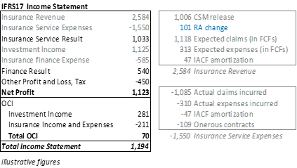
The two most common techniques adopted to derive the RA are the Cost of Capital (CoC) approach and the Value at Risk (VaR) approach. As it appears to be quite complicated translating a confidence level into a CoC value (for the avoidance of doubt, the 6% CoC under SII is not equivalent to a quantile of 99.50%), many companies are opting for the second technique, deeply discussed in the following. The higher the RA, the higher the uncertainty around the projections. The article also describes the pros and cons of having a high or low value of Risk Adjustment and how its variation can be split into one part concerning the services already provided, and released to the IS, and another part concerning the future services and counted for in the CSM. Indeed, as shown by the following picture, this RA change, together with the Expected Claims, compares to the Actual Claims, to capture the non-economic variance.
To adopt a VaR approach, the undertaking shall define the perimeter of risks to analyse, the confidence level at which the VaR is measured, and its time horizon: indeed, the remaining lifetime of the contract must be considered when deriving a provision for the uncertainty of non-financial risks. A possible calculation of the RA can be run following these steps, from the bottom to the top:
- the RA is defined as a n-years VaR, with n indicating the remaining lifetime of the pool of contract
- the n-years VaR is derived from the 1-year VaR
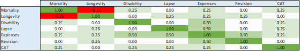
- the 1-year VaR is derived by aggregating 1-year univariate VaR (one for each risk considered)
this can be done, for example, by means of the SII LUR correlation matrix
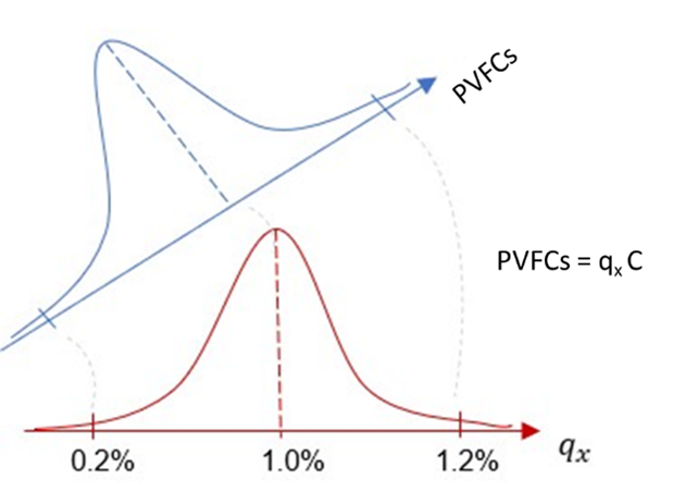
- each univariate 1-year VaR is defined as the change in PVFCFs (stressed – base) when a certain risk is stressed to a given confidence level, based on its distribution.
This methodology holds under the assumptions that
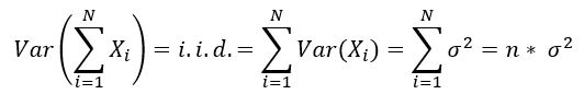
- during the remaining n years of projection, the shocks of the underwriting risks are independent and identically distributed (i.i.d.), for instance with a Gaussian distribution
- the distributions of the shocks and their confidence levels are transformed into distributions of stressed PVFCFs, as shown by this trivial example of direct linear dependency to the mortality risk
The outlined methodology is based on the following principles
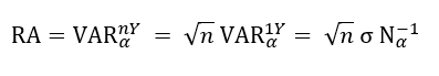
- the RA measures the uncertainty (variability) around the PVFPs value in the following n years
- the uncertainty with a given confidence level a is measured as the VaR of PVFCFs returns (i.e., variations in its value) that are i.i.d. and distributed as Gaussians
- the PVFCFs returns are directly linked to the shocks of the risks, that are distributed as Gaussians and whose value can be derived from the stress level defined by the SII directive (with an exception for the CAT risk, that can be kept at the SII level, for the sake of prudency)
This drives to the conclusion that
The idea behind the formula is that
- the (multiperiodic) RA under IFRS17, similarly to the (one-period) RM under SII, is a provision for the uncertainty around the estimation of the underwriting risks, therefore a cushion to absorb unexpected changes in the PVFCFs driven by unexpected changes in the underwriting parameters
- under SII the SCRRU measures the reduction of OF in a stressed combined scenarios with stresses pushed at a confidence level of 99.50% (1 every 200 years)
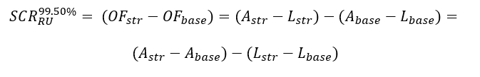
- in each univariate dimension of underwriting risks (aggregated by the means of a correlation matrix), the Assets (A) stay the same and the univariate capital requirement corresponds to a change in Liabilities (L)
- the Liabilities (L) establish a value (a price) for the insurance contract and the SCRRU provides a change in that price, so a return when compared to the base Liability value: for example, given Lbase=100 and Lstr=110, the SCRRU is defined as delta(L) = 110-100=10, corresponding to a simple return of 10% or, equivalently, to a logarithmic return of 9.53%. Logarithmic returns are generally adopted for their useful properties of being summed up (10%+10%=20%), that does not hold when linear returns are considered
- the prices are generally modelled with Lognormal distributions (always positive), while the returns with Gaussian distributions (bidirectional: positive or negative); similarly, we can consider PVFCFs (almost) always positive and changes in PVFCFs to be both positive and negative
- the RM can be seen as a CoC
- holding the SCR is a cost for the undertaking, with the SCR that decreases in a runoff portfolio
- the RM expresses a cumulated cost of capital requirements, with the CoC (6%) hinting a return those capitals may have yield if invested elsewhere
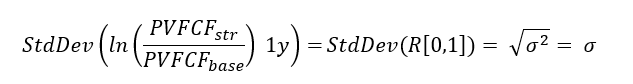
The mathematical background to the VaR derivation is given by the following
- n years of projections are considered for the remaining duration of the portfolio
- the prices, distributed as Lognormal, indicate the PFVCFs values, while the returns, distributed as Gaussians, indicate the variations (returns) of those prices, driven by the shock of the underwriting parameters
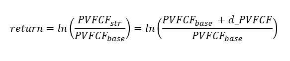
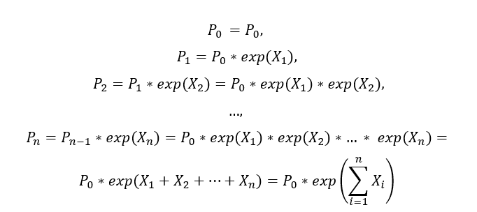
- during the n years of projections, the undertaking faces shocks, i.e. (PVFCF_str/FPFCF_base) returns Xi, independent and identically normally distributed
- the prices, the PVFCF values, change because of these shocks
with
- PVFCFs changes (logarithmic returns)
- each PVFCFstr corresponds to a shock (a misestimate on a certain UW risk parameter)
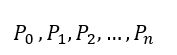
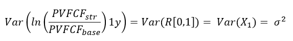
- the 1-year ln(PVFCF_str/PVFCF_base) corresponds to the first-year return R[0,1] = ln(P1/P0) = X1
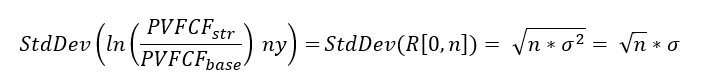
- the n-years corresponds to the n-years return R[0,n] = ln(Pn/P0) = sum(Xi)
- variance of PVFCFs logarithmic returns
- measures how much the stressed PVFCF values differ from each other, where each one derives from a certain shock (misestimate on the calibration of a certain parameter)
- the 1-year variance of the logarithmic returns is defined as
- the variance of the logarithmic returns corresponds to
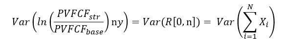
that under the independence hypothesis can be written as
- standard deviation of PVFCFs logarithmic returns
- easier to interpret having the same magnitude as the returns (for instance given the standard normal distribution, the 95% of the observations fall within 1.96 standard deviation)
- 1-year standard deviation
- n-years standard deviation
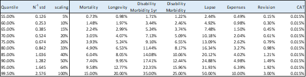
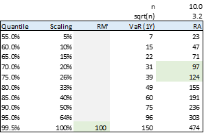
A sensible confidence level can be derived by targeting the value of the SII RM, where the only SCRRU part is considered (RM’). Indeed, when performing the RM’ calculation (in this illustrative example equal to 100), the undertaking considers the costs of the projected 1-year VaRs, each one defined with a confidence level of 99.50%. By scaling the first 1-year VaR (in this illustrative example equal to 150) back to smaller confidence levels and by multiplying these outcomes by the squared root of the remaining duration, the undertaking can define a sensible quantile by targeting these results to the value of adjusted RM’ (in this illustrative example, somewhere between 70% and 75%).
The IFRS17 principles permit diversification in the RA, that can occur because of the interaction between risks (considered in this article by the usage of a correlation matrix) and because of the granularity chosen to carry out the calculation (contracts, UoA, portfolios or entity level). As the principle requires to group contracts in UoA when they have similar risks and are managed together, it seems reasonable to diversify within the UoA, with a diversification effect that is likely to be small, as the contracts are exposed to similar risks. Still, an undertaking may claim to manage non-financial risks across different portfolios all together and move the RA calculation to a less granular level; it may also claim that these risks are reinsured and can be treated at entity level. In case the latter options were chosen, the undertaking should in any case find a way to reallocate the total RA amount to the single UoA the portfolio is composed of.
The author believes there is no point in gaining an additional diversification benefit and in trying to lower the RA. Even if a higher RA at transition corresponds to a lower Net Asset Value, it can be released in the IS for what concerns the current services (increasing the IS result) and helps in balancing out deviations between expectations and reality from time to time.
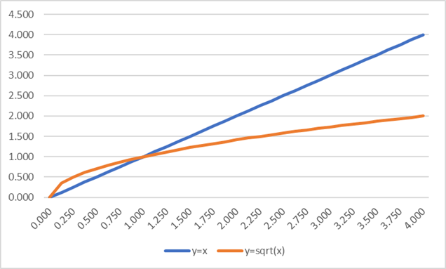
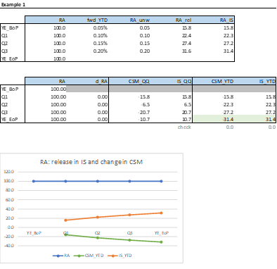
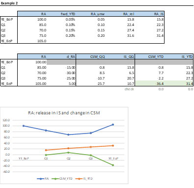
Following the definition of RA as an n-years VAR, the undertaking can assume that, over an evaluation period, the expected RA release in the IS is equal to the 1-year VAR defined at the beginning of period. When a “year to date” (YTD) evaluation is performed, the release is given by the YTD VaR, with YTD<1 year, and a consequent big release in the first quarter and smaller releases in the following ones, driven by the path of the square root function, that lays above the bisector (y=x) till x=1. When it comes to the n-years VaR definition derived from the 1-year VaR, the scaling factor, always defined by the square root of the remaining duration, becomes much smaller than the outstanding time, as sqrt(x) << x for x>1.
The following illustrative examples clarify how the RA movement can be split into the two components affecting respectively the IS, for services already provided during the year, and the CSM, for future services. At the end of the year (EoP), the sum of the two components must be equal to the change in RA registered over the year. Indeed, in Example 1, -31.4+31.4 = 0 = 100-100, while in Example 2, -36.4+31.4 = -5 = 100-105. The RA released in the Income Statement is given by the theoretical RA to release, as previously defined, minus the RA unwinding, calculated by the means of the forward rates defined at the beginning of the period (BoP). As it is easy to notice in Example 1, where a constant RA is given, what is released in the IS must be offset by a reduction of the CSM.
Reference:
- IFRS – IFRS17 Insurance Contracts and Amendments to IFRS17, May 2017 and following
- IFRS – Transition Resource Group for IFRS 17 Insurance Contracts, September 2018
- Silvia D.A., Annalisa Iacobone – IFRS17 is coming soon, November 2021

