Under Solvency II (SII), insurance and reinsurance companies have to evaluate their assets and liabilities following harmonized principles, among which the discounting of the liabilities cash flows through a risk free interest rates yield curve, that EIOPA has been publishing on a monthly basis since February 2015. The Authority does not state anything else regarding the future evolution of the risk free yield curve or the volatility it should show, which count a lot in the determination of the liabilities value.

If the liabilities were characterized by having no optionality, their present value could be easily calculated discounting the cash flows though the deterministic yield curve provided by EIOPA; in truth, insurance products usually offer a guarantee on a minimum level of return credited to policyholder fund. This optionality must be priced in a risk neutral framework, likely making use of Monte Carlo simulations. Whatever model is chosen to project the shape of the interest rates in the future, it must satisfy the risk neutrality principle (i.e. all the assets are expected to earn, on average, the risk-free rate). Roughly speaking, this means that, if we consider an asset that is worth X euros in t=0 and capitalize and discount it over the N paths of the projected interest rates, the average value of the N evaluations should be X. Although, Liabilities cash flows are not that simple and the volatility of the projected rates plays an important role when defining the value of the optionality they embed. The Interest Rate (IR) model adopted is calibrated such that the projected interest rates are Market Consistent (MC), that is, capable of replicating some Implied Volatilities (IVs) quoted in the market. The question is: which IV shall be targeted? It is worth noticing that we move from talking about the volatility of the interest rates, used to price the optionality (and therefore the IV) of the liabilities to a different IV, that comes from the market, from completely different types of options. When thinking about the market, another important piece of information is that the price of an instrument is unique, while its IV depends on certain assumptions: it is implied by a specific formula. Another key element is that prices are the unique quantity definable via Monte Carlo simulation, while IV shall be derived from the former.

The SII regulation does not provide any answer and the choice is left to the insurance and reinsurance undertakings, which can select the IR model they prefer and its market target for the calibration purposes. Actually, the Standard Formula does not even consider the IR volatility as a risk.

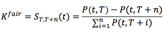
The IVs quoted in the market are those of the Cap, Floor and Swaption contracts, all the three being defined over an Interest Rate Swap (IRS).The IRS is a derivative instrument where two parties agree to exchange IR cash flows from a fixed () to a floating () rate, or vice versa. The IRS is called payer/receiver when the fixed rate is paid/received. The fixed rate that makes the contract fair is called forward swap rate and is equal to:

where is the time when the contract starts and the number of years it lasts.

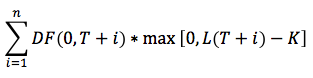
Caps and Floors can be respectively seen as options on a payer/receiver IRS, where the money exchange is set in favorable circumstances only. The present value of the payoff of a Cap is:

Caps can be used for hedging purposes when one is debtor of the floating rate . Indeed, when holding such a contract, the whole exposition becomes , that does not exceed the fixed rate . Caps and Floors are made up of sequences of Caplets and Floorlets, each one defined over a certain époque and referred to a certain forward rate. A Cap contract is said to be ITM (In), ATM (At) or OTM (Out of The Money) when K is respectively <, = or > than the fair value, and the difference between K and the fair value is called moneyness, so

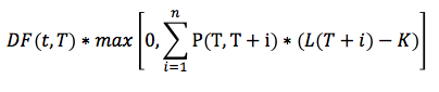
A payer/receiver Swaption contract is an option granting its owner the right but not the obligation to enter in into an underlying payer/receiver IRS of tenor . The actual value of a payer Swaption is:

Because of the Jensen inequality, this value is never grater that the Cap correspondent one. Likewise the Cap, a payer Swaption is said to be ITM, ATM or OTM when the strike K is respectively <, = or > than .

Until the recent past (say, before the negative rates appeared), both Caps/Floors (considered as sum of Caplets and Floorlets) and Swaptions were priced using the Black formula, supposing a lognormal distribution respectively for the forward rates and the forward swap rate. Although widely used in the market, the two pricings were incoherent, being the forward swap rate defined as a weighted average of the forward rates and the being the sum of aleatory variables with lognormal distribution not lognormal distributed (i.e. the two assumptions on the distributions of the rates cannot hold true together). As the price of a Swaption depends on the forward swap rate, knowing the volatilities of the single forward rates is no longer sufficient for the evaluation and information about the forward rates joint distribution and the correlation between different maturities are needed. Because their price embeds more information, Swaption contracts are often preferred to Caps when setting the market target for the calibration of the IR models.

Given a unique price of a Swaption, there are three types of IV quoted in the market, based on different assumptions on the distribution (Lognormal, Displaced Lognormal or Normal) of the swap forward rate:

• LN-SIV are defined as a relative change of the forward swap rate (bigger changes for higher YC)

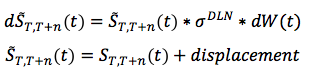
• DLN-SIV are defined as a relative change of the displaced forward swap rate

• N-SIV are defined as an absolute change of the forward swap rate, independent of its level

All the three are linked by the value of the underlying forward swap rate and, roughly speaking, there are 2 order of magnitudes between the former and the latter. Even though the relationship is not given by a simple rescaling and it is not linear, a good approximation to keep in mind is:

The recent past market environment, characterized by a number of tenors whose rate was negative, has questioned the use of LN-IV: negative/close to zero forward swap rates turn into not defined/extreme IV, which make the calibration of any IR model very challenging and potentially inaccurate.

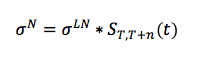
N-IV has started to catch on, with the additional benefit of mitigating the distortion that comes from applying a market IV to a Yield Curve (YC) that is different from the market one. Indeed, the IV quoted in the market refer to the market swap YC, while the IR models used for the liabilities evaluation are based on the published EIOPA YC (much higher on the long term due to the convergence to the UFR). The misalignment of applying a certain IV (that refers to the market YC) to a higher YC (the EIOPA one) is exacerbated when LN-IV are adopted, as they are proportional to the level of the rates. The usage of N-IV in place of LN ones helps in taming the volatility embedded in the projected rates, that affects the TVOG, normally increasing the BEL value. The following picture clarifies the statement, by comparing the market ATM LN Swption IV (implicit in the market rates) to those derived from the N-IV when the EIOPA YC is used: the latter are smaller because, given the same N-IV, a higher rate appears as denominator.

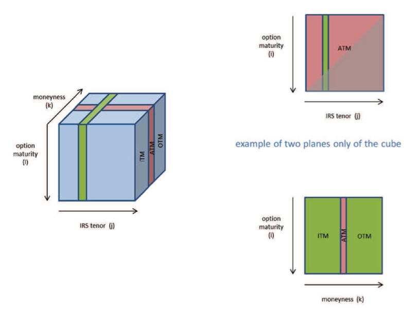
After having concluded that Swaptions are more exhaustive than Caps and, in this context, N-IV are more appropriate than LN-IV, a question is left: when calibrating an IR model, which data shall be considered as target among all those available for the Swaption N-IV (N-SIV) cube (option maturity , IRS tenor , moneyness) at a certain reference date?

Let’s try not to forget the original goal: determining a value for the Liabilities, that embed a degree of optionality, priced via Monte Carlo methods. The market data chosen as target drive the calibration of the IR model chosen and, in turn, the projected rates and their distribution. Different sets of projected rates give origin to different liability values. Setting a certain target is nothing else than deciding on the properties the projected rates should have, including their volatility, keeping in mind that the IV of the liabilities will not be equal to the IV of the Swaptions as the liabilities are not Swaption contracts.

Being the N-SIV quite smoothed, there is potentially no contraindication in setting the whole SIV cube as target but the runtime needed to carry out the IR model calibration: it is a matter of balance between calibration speed and fitting accuracy, which also depends on the IR model adopted. Deciding on which data to consider introduces a degree of subjectivity and exposes one to the risk/benefit of choosing some points rather than others. What if the others matters more? On the other hand, along with reducing the runtime, the selection of a subset of data may help in discarding unrepresentative or inaccurate data points, not consistent with the surrounding ones.

Once the relevant data have been chosen, the last question is: shall they all be weighted the same way or should some of them count more than others? The easiest possibility is to assign uniform weights to all the points considered, while a more subjective one is to decide on which SIV triples should count more. There is no contraindication of going for the first choice, while the latter introduces again a degree of subjectivity. A possibility for defining a not uniform weighting scheme would be to derive it from the liabilities’ profile, but it would be a more complex approach, less stable over time and subject to introducing sensitivity between rates levels and volatilities (the liability profile depends on the level of the rates and so the derived weights, which will drive the next calibration, like the tail wagging the dog). In addition to that, one should remember that there is no direct link between liabilities and Swaption contracts: the IV quoted in the marked for the Swaptions are not becoming IVs for the liabilities.

Having said that, in case liability driven weights was still the favorite option, an insurance company should define a parallelism between the financial optionality and that embedded in insurance products to derive the option maturities, IRS tenors and moneyness it is more exposed to. To this aim, only contracts with of a minimum guaranteed rate shall be considered. A “with profit” contract, where the policyholder has the right to get a minimum guaranteed rate in case of lapse/death/maturity, could be compared to a Long European Swaption as the policyholder may chose a fixed payout at the end of his contract or a variable benefit if he takes the money and invests it at the risk-free rate; from the perspective of the insurance company, this contract would be comparable to is a Short European Receiver Swaption. One can think of:

• the option maturity (T) as the time in which the policyholder can decide to leave the contract
• IRS tenor (n) as the residual time since the policyholder has left the contract till its original maturity
• the moneyness of the option (r_mg) as the difference between the minimum guaranteed rate (moneyness) and the swap forward rate S(T,T+n). In a market environment characterized by low yields and high guarantees, the liabilities would be more exposed to OTM Swaptions on the short term (a rational policyholder would prefer to stay in the contract and get the minimum guaranteed rate rather than reinvest the benefit in the market at the risk-free rate, which is lower) and to ITM Swaptions on the long term (when the market rates are higher than the guaranteed one).

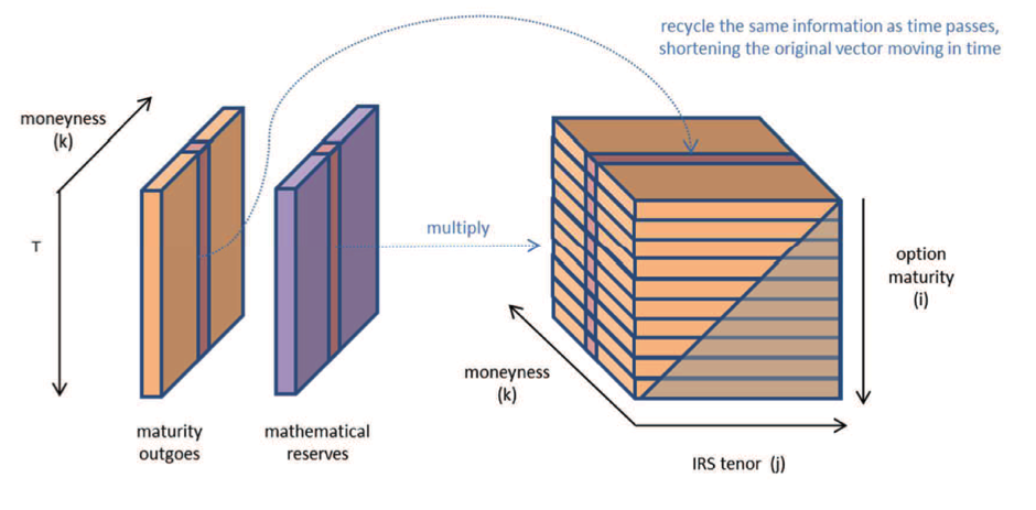
To put into effect this parallelism between insurance policies and financial contracts, one needs derive a 3D matrix (T,T+n,moneyness) starting from a 1D projection of mathematical reserves and outgo cash flows for the maturity only CF(t,MAT.OUT). The mathematical reserves are used as the best proxy of the amount of money the policyholder will get in case of lapse (exercise of the option), while maturity outgoes are considered being the only outgo cash flows where the policyholder can exercise an option (neither death cash flows are considered as the policyholder cannot decide to die/survive, nor annuity cash flows are, because, when paid, they correspond to a decision already made by the policyholder – staying in the contract and not leaving getting a lump sum).

• both V(t) and CF(t,MAT.OUT) can be split by r_mg, from which one can derive the moneyness (that gives the 3rd dimension)

• given a certain r_mg, to transform the 1D projection into a 2D matrix one has to “recycle” the data “moving in time”
• the first dimension (T) is naturally given by the “move in time”
• the exposure of the Liabilities to the IRIV risk is given by the amount of mathematical reserves that the policyholders can withdraw at that time (T), given the lapse rate as the base one

• at each (T), the second dimension (T+n) is given by the amount of contract in place at time e that are expiring in (T+n) – one moves in time considering for each row (i+1) a subset of the data used in (i), removing the first element

As the SIV cube does not include all the possible triples, the data without a correspondence have to be assigned to the nearest existing labels (e.g. tenor 6 is split equivalently to tenor 5 and tenor 7), in a “condensation” process. Even though it is be possible to identify the whole cube, the entries may be further condensed into a limited number of triples, which have been defined as target.

As already stated, the parallelism between financial and insurance options is just a parallelism that undergoes a number of simplifications, among which:

• ignoring additional payments on top of the minimum guaranteed amounts (that happen because of the profit sharing) as well as fiscal benefits or penalties in case of early surrender
• the surrender date is not set at maturity only: policyholders can surrender at any time until maturity (it would be more similar to a Bermudan option rather than to a European Swaption)
  • it is not exactly clear whether an insurance contract shall be addressed as payer or receiver option: looking at the payoff, the payer label would fit more (max(0,L-K) ), but from a definition perspective the policyholder actually receives from the insurance company a fixed amount, that than exchanges with a third party (the market).