
Following the overview provided in [5] “IFRS17 is coming soon”, this article focuses on a potential definition of Illiquidity Premium (IP) that appears to soften the so-called Bow Wave effect. Given a single value of IP, the author presents an alternative application to the risk-free rates other than the parallel shift, that reduces the gap between Real World and Risk Neutral evaluations, without introducing any bias: a mathematical and graphical proof is provided to show the equality of capitalization of the underlying volumes of reserves, that always reach the same value.
IFRS17 takes a longer-term view than IFRS4, immediately covering all the losses and postponing the profit profile, with this second feature driven by an unintended effect known as “Bow Wave”. For contracts where the VFA is used, the Bow Wave effect raises from the impact of Real Word (RW) returns on the unlocking of the Contractual Service Margin (CSM) in Risk Neutral (RN) projections.
The CSM is determined at initial recognition as the expected unearned profit embedded in the insurance contracts, based on an interest rate curve called locked in curve; the “unlocking of the CSM” indicates the adjustments applied to its value from time to time to offset the impacts of changes in the FCFs (Fulfilment Cash Flows) related to future services. The new accounting standards foresee that the CSM is amortized over the life of the contract and released into the P&L to best reflect the services already provided and the remaining duration: part of the CSM shall be released from reporting period to reporting period by considering the difference between the actual and expected service provided in the current period together with the expected service estimated for future periods, following an amortization pattern defined by the CU (Coverage Unit), that should represent a measure for the service delivery.
In a RN projection, on average, nothing can be earned more than the risk-free rate, however, in the RW, insurers expect to earn some excess of interest, often called “risk premium” or “expected spread”. If this “over-return” exists (it is positive), the IFRS17 principles state that the part belonging to the SH (Share Holder) shall be added to the CSM and released over the remaining duration. When the over-returns are systematic, the adjustments lead to a delay in the profit recognition, cumulate over time and, figuratively[1] speaking, generate a “Bow Wave” (BW) of excess of interests. A systematic delay of profits is not in line with the purpose of IFRS17, but, unfortunately, no patches have been hinted yet by either the standards or the IASB, albeit a solution must be found. Avoiding the BW effect means, in other words, having a release of CSM comparable with the one of a hypothetical CSM defined at inception and embedding all the future expected over-returns. This can be achieved in three possible ways (that can be potentially combined):
- proper Illiquidity Premium
the idea is to define an IP that pushes the RN projection towards the RW one
- CSM adjustment
the idea is to increase the CSM release by the SH share of excess of investment returns
- modified CU
the idea is to consider the over return in the definition of CU
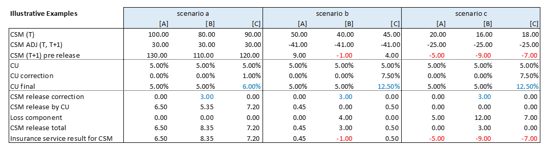
When [B] or [C] are chosen, the insurer should derive both the difference between the distribution of RW and RN returns in relation to the result of the reporting period (considering all the different asset classes, such as government and corporate bonds, equity, real estate, other investments) and the portion belonging to the SH (the SH share). In case of [B], the adjustment to the CSM can be either calculated by adopting a simplified approach, where the RW over-return of the investments is multiplied by a share derived from the experience, or by comparing the PVFP (Present Value of Future Profits) of two simulations, respectively run under the RN and RW measures. The table below provides an illustrative example of the CSM release, adopting, one at a time, the solutions outlined above, in different possible scenarios.
The Author believes that [A], compared to [B] and [C], provides a (at least partial) cleaner solution to the problem, avoiding further adjustments to the CSM release. A possible implementation is discussed in the following.
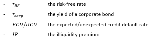
As stated by the principles, the discount rates adopted to determine the FCFs shall both reflect the level of current interest rates and the illiquidity characteristic of the liabilities, to counterbalance the credit effect on the asset side. The discount rates can be defined following a bottom-up or top-down approach, that should lead to the same result: in case of spike in the credit spreads, the former would raise the risk-free yields by a proportionate Illiquidity Premium (IP) and the latter would decrease the portfolio yields by a portion of the credit risk. Under the bottom-up approach, an IP is added to the risk-free rate to reflect the illiquidity characteristics of the insurance contracts; under the top-down approach, the full market value yield on the relevant assets is deducted by its credit risk component, without deduction in respect of its illiquidity component. In theory, both methods should be equal. Indeed, by indicating with
the spread of a corporate bond (i.e. the difference between its yield and the risk free one) is given by

and, rearranging the terms, we have
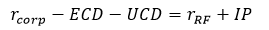
or, in other words
top-down approach = bottom-up approach
IFRS17 is a principles-based standard, that sets out a guidance, without explicitly establishing the rules for discounting: to define their own approach, insurers can consider various possibilities, adopt a relevant judgment, and agree with their auditors. Albeit no formulas are indicated, let us recall paragraph 36, that describes how to define the discount rates, that shall:
- reflect the time value of money, the characteristics of the cash flows and the liquidity characteristics of the insurance contracts
- be consistent with observable current market prices for financial instruments with cash flows whose characteristics are consistent with those of the insurance contracts, in terms of, for example, timing, currency and liquidity
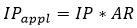
- exclude the effect of factors that influence such observable market prices but do not affect the future cash flows of the insurance contracts.
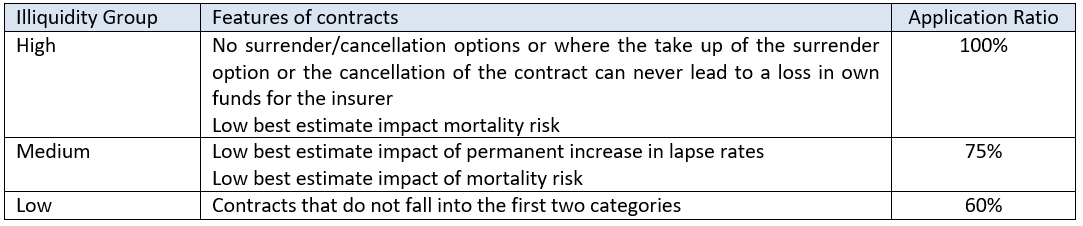
The Liquidity usually indicates the ease with which assets can be converted into cash without affecting their market price, being the cash the most liquid asset (it can be traded to buy anything). A feature that influences the liquidity of Liabilities is the change in their duration when stressed events occur: the more sensitive the duration is to stressed scenarios (such as a mass lapse), the more liquid is the contract (indeed UL products are more liquid than SAV ones). The comparison between the durations of the liabilities and the assets backing the liabilities can provide an indication of the share of the assets IP that can be applied to the liabilities. This share is referred to as the Application Ratio (AR).
Paragraph B79 introduces a guidance on how to assess the liquidity of insurance contracts by considering the features of the products, that can generate an exit-value, an inherent value, and an exit cost, all these three components influencing the liquidity of the product:
Yield curves reflect assets traded in active markets that the holder can typically sell readily at any time without incurring significant costs. In contrast, under some insurance contracts the entity cannot be forced to make payments earlier than the occurrence of insured events, or dates specified in the contracts.
Some examples are provided in the following
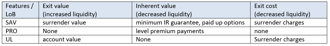
This view is aligned to what EIOPA has proposed in its consultation paper [3], when defining the degree of liquidity based on the terms and conditions of insurance contracts
A similar idea is also shared by the MCEV (Market Consistent Embedded Value): the principles state that “A liability is liquid if the liability cash flows are not reasonably predictable”. When a liability is illiquid (liquid), the corresponding cash flows are (not) predictable, and the insurance company is (not) willing to hold the backing assets to maturity to target a higher investment return, given by the risk-free rates plus a liquidity premium. When a “buy to hold” strategy is adopted, the insurer is not exposed to volatility of market prices and can therefore lock in the premium above the risk-free rate, that compensates the holder for locking up the investment for a long-term.
Finally, paragraphs B78-B85 highlight the key principles to follow for determining the liquidity premium:
- Maximize the use of observable inputs
- Reflect current market conditions
- Exercise judgment to assess the degree of similarity between the features of the insurance contracts and assets with observable prices and make further adjustments as needed
and paragraphs B78-B79 stress that discount rates shall exclude the credit risk, which is not a characteristic of the insurance contracts.
Therefore, to define the discount rate of the liabilities under the bottom-up approach, insures should
- derive an IP based on the portfolio of assets held (removing the credit risk)
- derive an AR either based on “buckets of illiquidity”, identified by the features of the products, or based on the level of assets and liabilities mismatch (duration gap)
- define the discount rate as
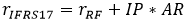
Albeit, theoretically, highly illiquid insurance contracts may be distinguished by rates of discount higher than the expected yield of the backing (less illiquid) assets, the AR is usually capped at 100%, to avoid this to happen. A sensible definition of AR may be
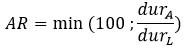
with dur_x indicating the duration of Assets (A) and Liabilities (L).
The bottom-up approach reminds the definition of the risk-free rates provided by EIOPA in the SII context, with the IP being like the VA (Volatility Adjustment), calibrated on the undertakings portfolios, rather than on an average European one and 65% being the AP. Such derivation would lead to a relatively small value of IP, comparable to the EIOPA VA, that would not solve the need of having a sensible RW CSM release.
The reason for that is the definition itself of the “gross” VA (i.e. before the application ratio), that is given by the sum of a government and corporate risk corrected spread components, with weights usually biased towards the first one, where the Risk Correction (RC) levels down or even exceeds the original spread. The RC is almost the same for all the portfolios, whether these belong to EIOPA or the entity, being defined over averages value of 30 years of history. An illustrative example is provided in the following table, where the EIOPA reference portfolio is compared to three illustrative entity specific portfolios
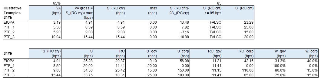
Such values are too low and do not reflect the liquidity of the liabilities at all. The Author believes there must be positive a correlation between the IP value and the Minimum Guaranteed rate offered by products; in fact, given the low level of interest rates the market is currently experiencing, insurance entities often invest in illiquid asset classes that can bridge the gap left behind by the fixed interest bonds, still satisfying the required level of cash flow matching. As a recap
- the IP measures the premium of illiquidity of the liabilities
- it cannot be measured over the liabilities, but it could be measured over a replicating portfolio of assets, that should exactly match the liabilities cash flows (even if it is common practice to look at the duration only)
- the assets baking the liabilities are a good compromise and the author believes that the IP shall be derived for alternative assets too, by means of the look through, as they are used to match the liability cash flows: high level of minimum guaranteed returns would not be sustained by investing in government and corporate bonds only with a reasonable duration. At the end of the day, a private debt can be comparable to a bond, with the difference that the money is lent to a firm not quoted in the regulated markets: there is for sure a credit risk to be removed, but the remaining IP will be quite high. The IP will then be the asset spread deducted of its risky component and it can be identified as the bid-offer spread.
The following charts compares the net flows of three illustrative types of portfolios
- guaranteed return of 4% and a duration of 10.6 years
- guaranteed return of 0% and a duration of 6.3 years (lower IP expected)
- guaranteed return of 0% and recurrent premiums, with the same duration as the first one, 10.5 years, that should be as liquid as the second one
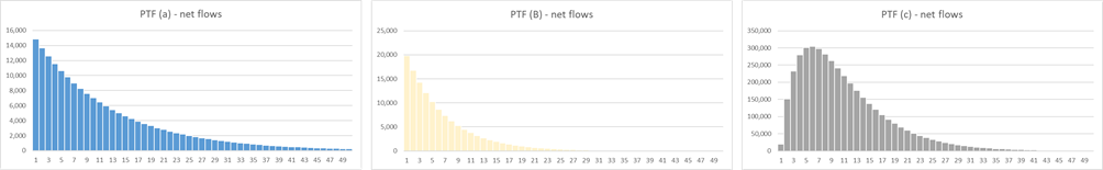
Despite having the same duration, the former and the latter portfolios are very different, with a) being highly illiquid, as few people would be willing to buy it, unless reducing its cost by including a premium for its illiquidity. In terms of cash flows, to replicate a) the company should hold assets at high yields, while c) can be managed with recurrent premiums and plain bonds.
Having defined the AR to apply to the IP, and the perimeter of assets from where it is derived, the Author presents its opinion on how the
can be added to the risk-free rates to reduce the BW effect. The Bow Wave tends to hit more in the first years of projections, when the risk-free rates are negative and the RW return is positive. The idea behind this approach is to increase as much as possible the coherency between the RN capitalization and discount of the volumes projected, where the capitalization applies a yield of the Segregated Funds (r_SF) that is comparable to a RW value, as it still embeds the Unrealized Gains and Losses (UGL), albeit being RN. The solution is to define an IP that changes over time, following the pattern of the UGL. Let us indicate with
The IP to apply to the risk-free rates is given by

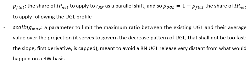
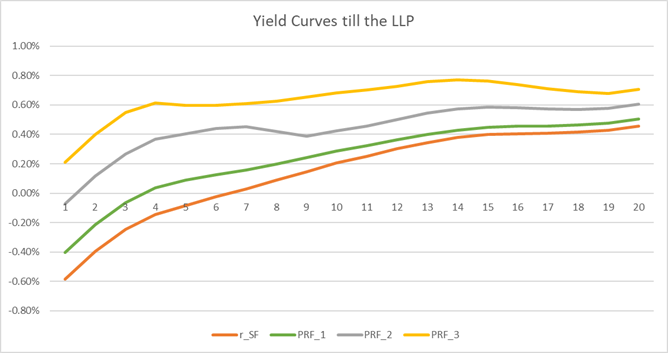
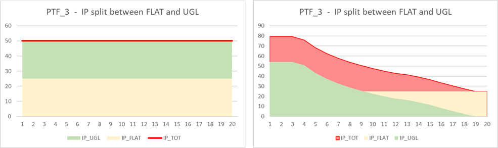
The following charts show graphically the idea behind the formulas: the total value of single IP that would be applied as a parallel shift to the risk-free curve over time is preserved and, instead of being flat, is split into a flat and UGL component. Three illustrative portfolios are compared, with a total IP of respectively 10bps (PTF_1), 30bps (PTF_2) and 50bps (PTF_3), and the parameters p_flat and scaling_max respectively set to 50% and 200%.
The two following charts clarify the decomposition of IP: in the former, the net single IP (red line) is applied as a parallel shift to the risk-free rates (the integral is given by the area of the rectangle), while, in the latter, the net IP (red area) is given by the sum of the two components (yellow, flat, and green, UGL), where the two areas equals those of the first chart, but the green one has a shape coherent to the UGL release. The total red area is the same by construction.
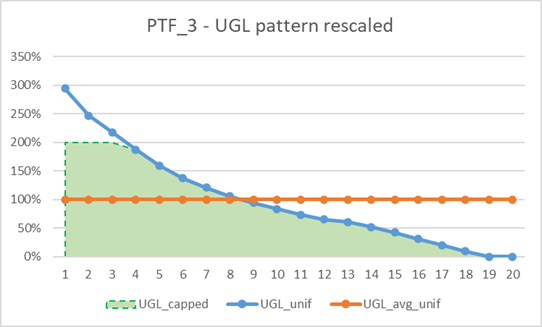
This graph shows the UGL value over time (blue line), compared to its average value (orange line), where they have both been normalized such that the average value equals 100%, to easily understand the application of scaling_max and the definition of the green area. The amount of UGL is not of interest, just their release shape is
The following charts show some sensitivity analyses carried out on PTF_3 to outline the behavior of the final IP depending on the choice of the parameters p_flat and scaling_max: equal to 100% (or 0%) implies that no (or all) the UGL shape drives the IP application, scaling_max equal to 1000% (or 0%) describes a situation where no correction on the UGL release (or no UGL at all) is considered to define the final IP
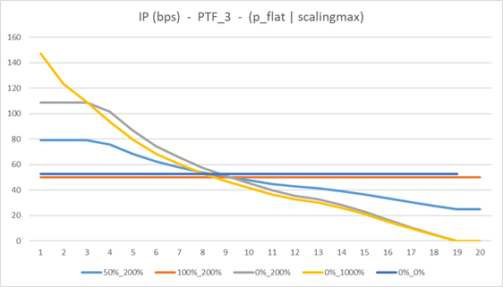
Some comments:
- the orange line (100%_200%, all flat) shows the starting point, where the IP application is coherent to the SII framework, where the VA is applied as a parallel shift to all the maturities
- the light blue line (0%_0%, all UGL with no possibility of considering any because of the cap) reverts to the orange one. They are not the same as the UGL exist till year 19, while the LLP start at year 20. The integral of 20 years is spread over just 19 years
- the blue line (50%_200%) is a meaningful choice in the author’s view
- the grey line (0%, 200%) is steeper than the blue line allocating to the UGL component all the area at disposal
- the yellow line (0%, 1000%) compares to the grey one, where the implication of not having any cap is shown: the UGL are massively released in the first years. It is also traces over the UGL release shape outlined above.
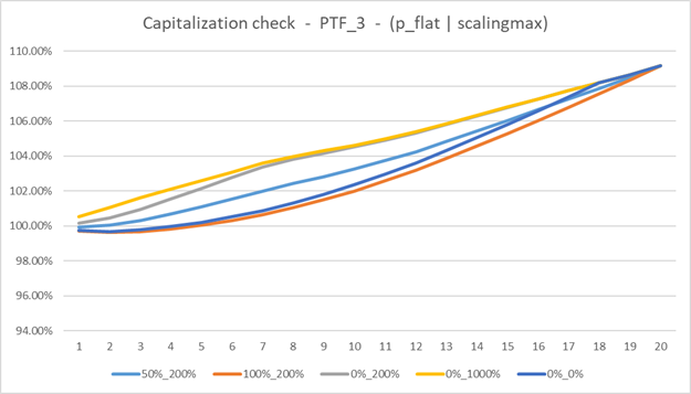
This final chart provides a proof of the convergency of the capitalization under these very different cases: the capitalization value is preserved as the integral is. This is the proof that the approach does not introduce any bias as no additional source of illiquidity premium is added: the total value is just spread out in a more sensible way, reducing the Bow Wave effect.
Reference:
[1] IFRS – IFRS17 Insurance Contracts and Amendments to IFRS17, May 2017 and following
[2] IFRS – Transition Resource Group for IFRS 17 Insurance Contracts, September 2018
[3] EIOPA – Technical specification of the information request on the 2020 review of SII, March 2020
[4] DAV – IFRS 17 for German life insurance, May 2020
[5] Silvia D.A., Annalisa Iacobone – IFRS17 is coming soon, November 2021
[1] A bow wave is the progressive disturbance propagated through the water because of the displacement by the foremost point of the ship, the bow, that moves faster than the waves. It defines the wake of the ship, that, view from above, is V-shaped.

