Since then, Binance joined the Internet and Mobile Association of India (IAMAI), which played a key role in overturning the ban, and noted explosive growth via WazirX…
The European Securities and Markets Authority (ESMA), the EU’s securities markets regulator, has submitted a response to the European Commission’s (EC) consultation on a new digital finance strategy for the European Union…
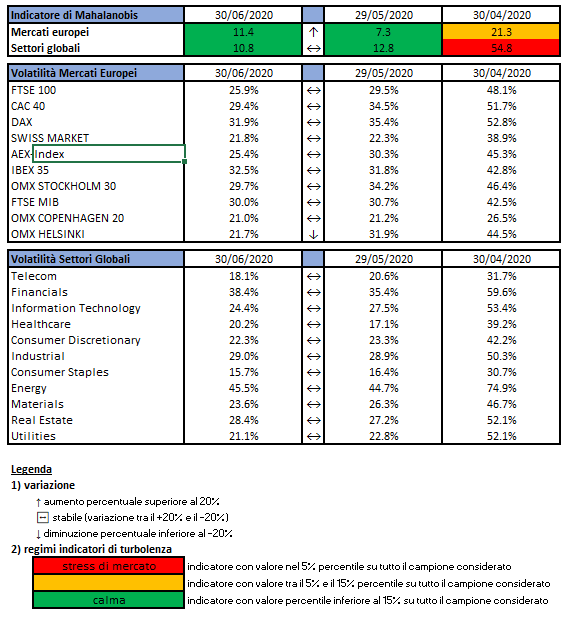
L’indicatore di Mahalanobis permette di evidenziare periodi di stress nei mercati finanziari. Si tratta di un indicatore che dipende dalle volatilità e dalle correlazioni di un particolare universo investimenti preso ad esame. Nello specifico ci siamo occupati dei mercati azionari europei e dei settori azionari globali.
Gli indici utilizzati sono:
Le volatilità riportate sono storiche e calcolate sugli ultimi 30 trading days disponibili. Per ogni asset-class dunque sono prima calcolati i rendimenti logaritmici dei prezzi degli indici di riferimento, successivamente si procede col calcolo della deviazione standard dei rendimenti, ed infine si procede a moltiplicare la deviazione standard per il fattore di annualizzazione.
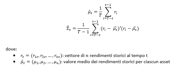
Per il calcolo della distanza di Mahalnobis si procede dapprima con la stima della matrice di covarianza tra le asset-class. Si considera l’approccio delle finestre mobili. Come con la volatilità, si procede prima con il calcolo dei rendimenti logaritmici e poi con la stima storica della matrice di covarianza, come riportato di seguito.
Supponendo una finestra mobile di T periodi, viene calcolato il valore medio e la matrice varianza covarianza al tempo t come segue:
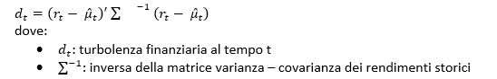
La distanza di Mahalanobis è definita formalmente come:
Le parametrizzazioni che sono state scelte sono:
Rilevazioni mensili
Tempo T della finestra mobile pari a 5 anni (60 osservazioni mensili)
Le statistiche percentili sono state calcolate a partire dalla distribuzione dell’indicatore di Mahalanobis dal Dicembre 1997 al Dicembre 2019 su rilevazioni mensili.
Disclaimer: Le informazioni contenute in questa pagina sono esclusivamente a scopo informativo e per uso personale. Le informazioni possono essere modificate da finriskalert.it in qualsiasi momento e senza preavviso. Finriskalert.it non può fornire alcuna garanzia in merito all’affidabilità, completezza, esattezza ed attualità dei dati riportati e, pertanto, non assume alcuna responsabilità per qualsiasi danno legato all’uso, proprio o improprio delle informazioni contenute in questa pagina. I contenuti presenti in questa pagina non devono in alcun modo essere intesi come consigli finanziari, economici, giuridici, fiscali o di altra natura e nessuna decisione d’investimento o qualsiasi altra decisione deve essere presa unicamente sulla base di questi dati.
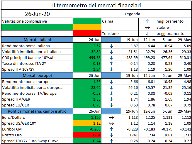
L’iniziativa di Finriskalert.it “Il termometro dei mercati finanziari” vuole presentare un indicatore settimanale sul grado di turbolenza/tensione dei mercati finanziari, con particolare attenzione all’Italia.
Significato degli indicatori
Rendimento borsa italiana: rendimento settimanale dell’indice della borsa italiana FTSEMIB;
Volatilità implicita borsa italiana: volatilità implicita calcolata considerando le opzioni at-the-money sul FTSEMIB a 3 mesi;
Future borsa italiana: valore del future sul FTSEMIB;
CDS principali banche 10Ysub: CDS medio delle obbligazioni subordinate a 10 anni delle principali banche italiane (Unicredit, Intesa San Paolo, MPS, Banco BPM);
Tasso di interesse ITA 2Y: tasso di interesse costruito sulla curva dei BTP con scadenza a due anni;
Spread ITA 10Y/2Y : differenza del tasso di interesse dei BTP a 10 anni e a 2 anni;
Rendimento borsa europea: rendimento settimanale dell’indice delle borse europee Eurostoxx;
Volatilità implicita borsa europea: volatilità implicita calcolata sulle opzioni at-the-money sull’indice Eurostoxx a scadenza 3 mesi;
Rendimento borsa ITA/Europa: differenza tra il rendimento settimanale della borsa italiana e quello delle borse europee, calcolato sugli indici FTSEMIB e Eurostoxx;
Spread ITA/GER: differenza tra i tassi di interesse italiani e tedeschi a 10 anni;
Spread EU/GER: differenza media tra i tassi di interesse dei principali paesi europei (Francia, Belgio, Spagna, Italia, Olanda) e quelli tedeschi a 10 anni;
Euro/dollaro: tasso di cambio euro/dollaro;
Spread US/GER 10Y: spread tra i tassi di interesse degli Stati Uniti e quelli tedeschi con scadenza 10 anni;
Prezzo Oro: quotazione dell’oro (in USD)
Spread 10Y/2Y Euro Swap Curve: differenza del tasso della curva EURO ZONE IRS 3M a 10Y e 2Y;
Euribor 6M: tasso euribor a 6 mesi.
I colori sono assegnati in un’ottica VaR: se il valore riportato è superiore (inferiore) al quantile al 15%, il colore utilizzato è l’arancione. Se il valore riportato è superiore (inferiore) al quantile al 5% il colore utilizzato è il rosso. La banda (verso l’alto o verso il basso) viene selezionata, a seconda dell’indicatore, nella direzione dell’instabilità del mercato. I quantili vengono ricostruiti prendendo la serie storica di un anno di osservazioni: ad esempio, un valore in una casella rossa significa che appartiene al 5% dei valori meno positivi riscontrati nell’ultimo anno. Per le prime tre voci della sezione “Politica Monetaria”, le bande per definire il colore sono simmetriche (valori in positivo e in negativo). I dati riportati provengono dal database Thomson Reuters. Infine, la tendenza mostra la dinamica in atto e viene rappresentata dalle frecce: ↑,↓, ↔ indicano rispettivamente miglioramento, peggioramento, stabilità rispetto alla rilevazione precedente.
Disclaimer: Le informazioni contenute in questa pagina sono esclusivamente a scopo informativo e per uso personale. Le informazioni possono essere modificate da finriskalert.it in qualsiasi momento e senza preavviso. Finriskalert.it non può fornire alcuna garanzia in merito all’affidabilità, completezza, esattezza ed attualità dei dati riportati e, pertanto, non assume alcuna responsabilità per qualsiasi danno legato all’uso, proprio o improprio delle informazioni contenute in questa pagina. I contenuti presenti in questa pagina non devono in alcun modo essere intesi come consigli finanziari, economici, giuridici, fiscali o di altra natura e nessuna decisione d’investimento o qualsiasi altra decisione deve essere presa unicamente sulla base di questi dati.
Il coefficiente della riserva di capitale anticiclica (countercyclical capital buffer, CCyB) per il terzo trimestre del 2020 è fissato allo zero per cento…
Questo sito utilizza cookie tecnici e di profilazione, propri e di terze parti, per garantire la corretta navigazione, analizzare il traffico e misurare l'efficacia delle attività di comunicazione.
Questo sito Web utilizza i cookie per migliorarne l'esperienza di navigazione. I cookie classificati come necessari, sono essenziali alle funzioni di base sito e vengono sempre memorizzati nel tuo browser. I cookie di terze parti, che ci aiutano ad analizzare e capire come utilizzi questo sito, vengono memorizzati nel tuo browser solo con il tuo consenso. Di seguito hai la possibilità di disattivare questi cookie. Tieni in conto che la disattivazione di alcuni di questi cookie potrebbe influire sulla tua esperienza di navigazione.
Necessary cookies are absolutely essential for the website to function properly. These cookies ensure basic functionalities and security features of the website, anonymously.
Cookie
Durata
Descrizione
cookielawinfo-checkbox-analytics
1 year
Cookie tecnico impostato dal plugin GDPR Cookie Consent che viene utilizzato per registrare il consenso dell'utente per i cookie nella categoria "Analitici".
cookielawinfo-checkbox-necessary
1 year
Cookie tecnico impostato dal plugin GDPR Cookie Consent che viene utilizzato per registrare il consenso dell'utente ai cookie.
CookieLawInfoConsent
1 year
Cookie tecnico impostato dal plugin GDPR Cookie Consent per salvare le scelte si/no dell'utente per ciascuna categoria.
viewed_cookie_policy
1 year
Cookie tecnico impostato dal plugin GDPR Cookie Consent che registra lo stato del pulsante predefinito della categoria corrispondente.
Analytical cookies are used to understand how visitors interact with the website. These cookies help provide information on metrics the number of visitors, bounce rate, traffic source, etc.
Cookie
Durata
Descrizione
_pk_id.gV3j99y0AE.0928
1 year 27 days
Cookie analitico impostato da Matomo e utilizzato per memorizzare alcuni dettagli sull'utente come l'ID univoco del visitatore
_pk_ses.gV3j99y0AE.0928
30 minutes
Cookie analitico impostato da Matomo di breve durata e utilizzato per memorizzare temporaneamente i dati della visita