Le evidenze del Rapporto CONSOB sulle scelte di investimento delle famiglie italiane per il 2018
La quarta edizione del Rapporto CONSOB sulle scelte di investimento delle famiglie italiane arricchisce l’articolazione delle edizioni precedenti attraverso la rilevazione di alcune variabili attitudinali che possono orientare i comportamenti di financial control, relativi a pianificazione finanziaria, gestione del budget familiare, indebitamento e risparmio [2].
Il financial control …
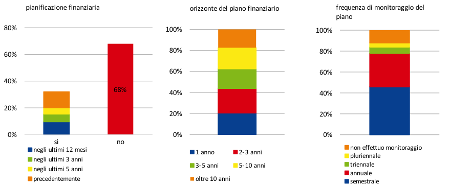
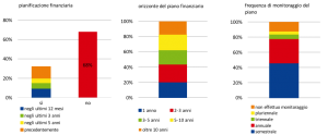
La gestione delle finanze personali e del bilancio familiare dovrebbe idealmente collocarsi nell’ambito di un processo strutturato che, nel solco di una sorta di ‘filiera’ del risparmio, parte dalla pianificazione finanziaria e dal budgeting per passare alle decisioni di risparmio e impiego dello stesso fino a concludersi con il monitoraggio e con le eventuali, necessarie revisioni del piano finanziario. Questi comportamenti, che nel complesso concorrono a definire il cosiddetto financial control, sono ancora poco diffusi. Solo un terzo dei decisori finanziari italiani dichiara di avere un piano finanziario (prevalentemente pluriennale), che monitora periodicamente (Fig. 1).
Fig. 1. La pianificazione finanziaria
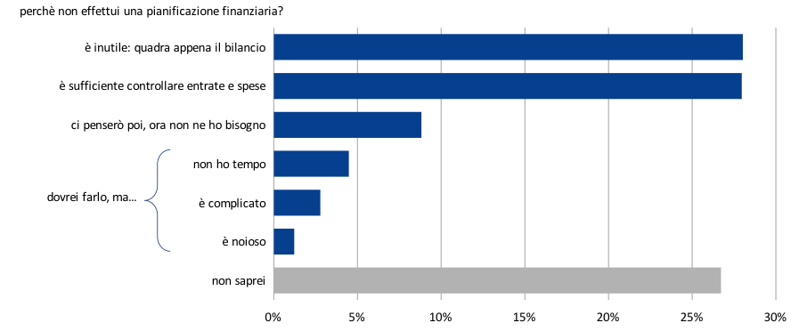
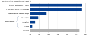
Fra coloro che non predispongono un piano finanziario, meno del 10% ne riconosce l’importanza, mentre circa il 65% lo ritiene inutile (Fig. 2).
Fig. 2. Fattori disincentivanti la pianificazione finanziaria
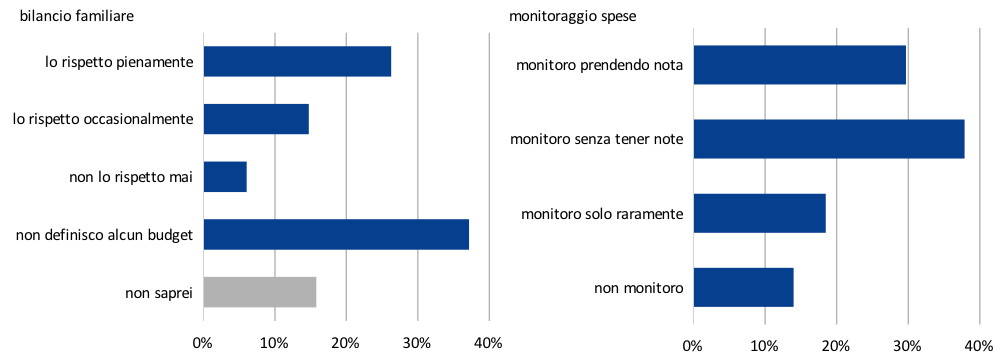
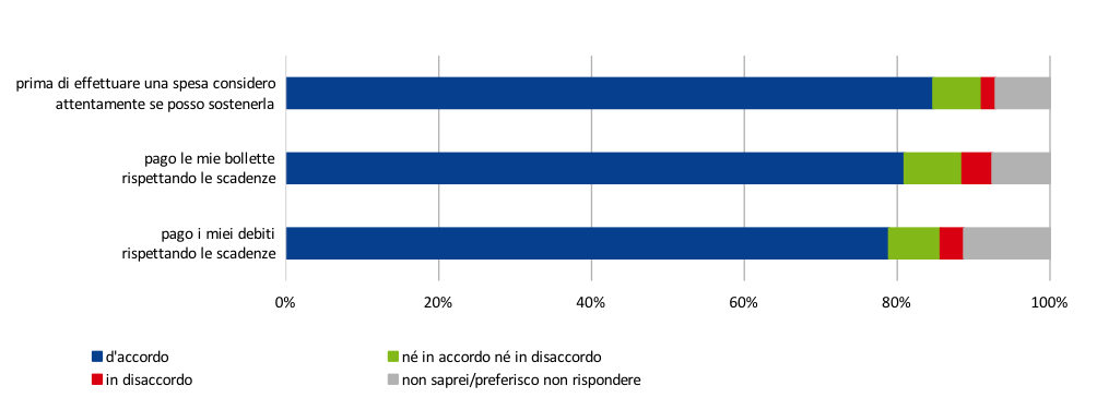
Rispetto alla pianificazione finanziaria, che presuppone la capacità di proiettarsi nel medio-lungo periodo, la definizione e la gestione di un bilancio familiare potrebbero essere potenzialmente temi più ‘salienti’ per chi deve gestire il denaro all’interno del nucleo familiare e per questo risultare più diffusi. Le evidenze disponibili, tuttavia, sembrerebbero smentire questa ipotesi. Solo il 47% degli intervistati, infatti, definisce e si attiene strettamente a un budget, a fronte di un 30% che tiene traccia scritta delle spese (Fig. 2). Il rimanente 40% che afferma di monitorare il budget lo fa in modo ‘non rigoroso’, anche se la maggior parte del campione riferisce di valutare gli acquisti attentamente (oltre a saldare le utenze a scadenza e onorare i debiti contratti, comportamenti questi che l’OCSE individua tra i financially savvy behaviour; Fig. 3) [3].
Fig. 3. Il bilancio familiare e il monitoraggio delle spese

Fig. 4. Abitudini in tema di spese correnti e impegni finanziari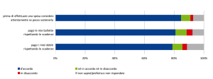
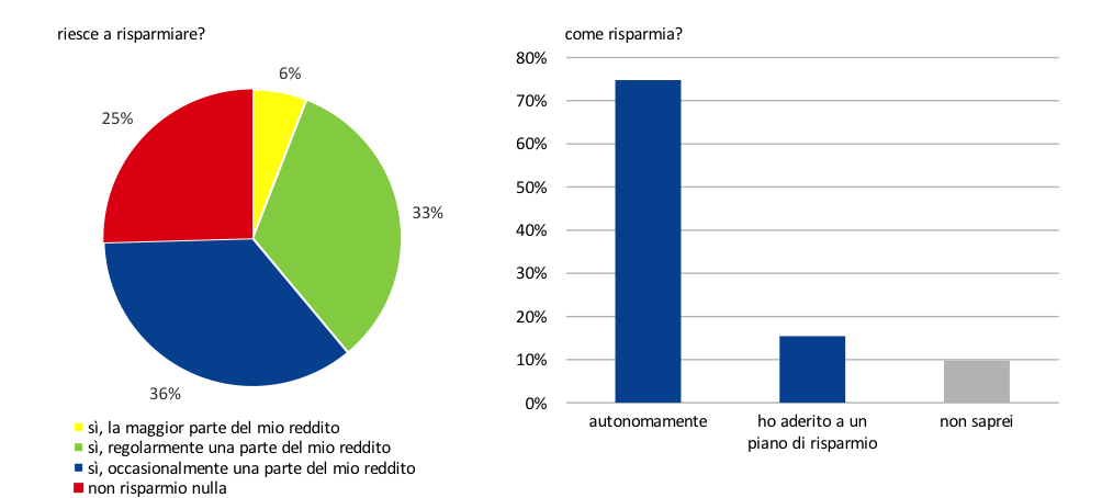
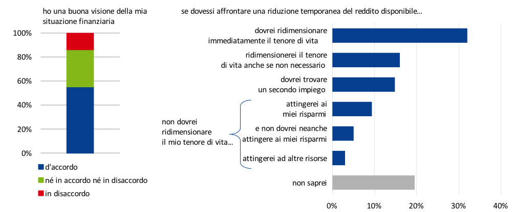
Pianificazione e controllo supportano la capacità di risparmio e favoriscono una visione chiara dello stato delle finanze personali. Per quanto riguarda il primo profilo, il risparmio regolare (che ricorre, soprattutto per motivi precauzionali, nel 40% dei casi circa) si associa positivamente con la propensione a pianificare (Fig. 5 e Report, Fig. 4.11).
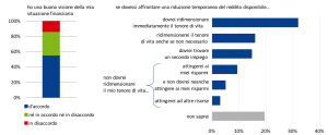
Con riferimento al secondo aspetto, un quinto del campione non saprebbe come affrontare una riduzione significativa del reddito disponibile (il 30% dovrebbe rivedere al ribasso le abitudini di spesa, mentre lo stile di vita potrebbe rimanere inalterato per circa un quinto delle famiglie, prevalentemente grazie ai risparmi accumulati; Fig. 6). Tra coloro che non sono in grado di valutare come affrontare un possibile shock finanziario negativo l’83% non pianifica e l’89% appartiene alle classi di reddito più basse. In generale, proprio coloro che trarrebbero i principali benefici dalla pianificazione, ossia gli individui meno facoltosi e più vulnerabili, non ne comprendono il valore aggiunto.
Figura 5. Abitudini di risparmio
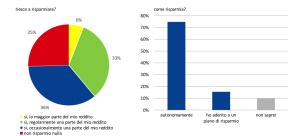
Figura 6. Resilienza percepita
A tal proposito, è interessante ricordare che i comportamenti di financial control si associano non solo a reddito e ricchezza finanziaria ma anche ad attitudini personali e conoscenze finanziarie.
… tra attitudini individuali …
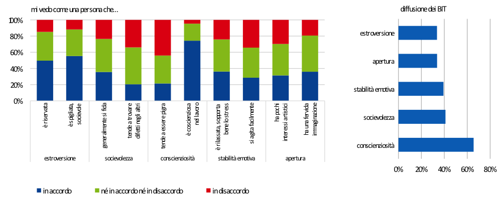
In linea con un nutrito filone della letteratura comportamentale, l’indagine 2018 amplia in modo significativo la rilevazione delle attitudini psicologiche che possono orientare le scelte economico-finanziarie individuali. Sulla base dell’autovalutazione dei soggetti intervistati, la maggior parte del campione dichiara di essere incline all’utilizzo di informazioni numeriche e ad attività cognitive impegnative (rispettivamente, 36% e 40%); auto-efficacia e auto-controllo sono diffusi presso il 46% e il 24% del campione, rispettivamente; sono molto frequenti, infine, la propensione all’ottimismo e la fiducia negli altri (rispettivamente, 35% e 29%); l’ansia finanziaria, infine, caratterizza nella sua maggiore intensità il 10% del campione e si colloca a un livello ‘medio’ per il 40% degli intervistati (Fig. 2.2 – Fig. 2.7). Un ultimo profilo riguarda le ‘personalità finanziarie’ (cosiddetti behavioural investors’ type), di cui l’Indagine dà conto per la prima volta evidenziando, tra i caratteri più diffusi, la prevalenza dell’attitudine ad essere coscienzioso (Fig. 7).
Fig. 7. I behavioural investors’ types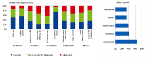
La preferenza per le informazioni di tipo numerico sembra essere più frequente tra gli uomini e tra gli individui con un livello di istruzione più elevato, al contempo maggiormente inclini ad attività cognitive impegnative. La propensione verso l’ansia finanziaria è più comune tra le donne e gli intervistati con un grado di istruzione più basso, mentre risulta correlata negativamente con la percezione di auto-efficacia e l’ottimismo.
Non sorprende che pianificazione finanziaria, budgeting e risparmio si associno positivamente all’inclinazione verso le informazioni numeriche e alla capacità di auto-controllo, mentre l’ansia finanziaria sembra essere un fattore deterrente (si veda la Figura 4.4 del Rapporto).
… conoscenze finanziarie …
Risulta meno scontato, invece, il fatto che i comportamenti di financial control si correlino positivamente non solo con le conoscenze finanziarie effettive ma anche con le conoscenze percepite. Nel Rapporto per il 2018, le conoscenze finanziarie effettive sono state rilevate, come di consueto, sia rispetto a nozioni di base (in linea con le big five utilizzate da Anna Lusardi e coautori in numerosi studi) sia rispetto a nozioni più sofisticate. Le rilevazioni confermano il basso livello di financial knowledge delle famiglie italiane: in media, un intervistato su due non è in grado di definire correttamente le nozioni di base; il dato scende a meno di uno su cinque nel caso di concetti avanzati (Fig. 3.1). Le conoscenze percepite sono state misurate in vari modi: sia ex-ante (ossia prima di mettersi alla prova con il questionario) in una duplice declinazione (rispettivamente, una generica autovalutazione del livello complessivo di dimestichezza con nozioni economico-finanziarie e una specifica autovalutazione della conoscenza dei temi oggetto del questionario) sia ex post, consistente nella stima del numero di domande alle quali si pensa di aver risposto correttamente. Il 40% del campione dichiara di avere, nel complesso, un livello elevato di conoscenze finanziarie, anche se la stessa valutazione ex ante riferita alle singole nozioni oggetto di indagine registra in genere percentuali inferiori (Fig. 3.2). Tale disallineamento tra conoscenze effettive e percepite trova conferma anche nell’auto-valutazione ex post (Fig. 3.3 e Fig. 3.4). Il quadro delle conoscenze finanziarie si completa con la cosiddetta risk literacy, definita con riferimento alla familiarità con specifici prodotti finanziari e alla capacità di valutarne il rischio relativo. Tra gli strumenti più conosciuti si annoverano i titoli di Stato (indicati dal 54% degli intervistati), mentre solo il 10% del campione è in grado di ordinare correttamente alcune opzioni di investimento per livello di rischio (Rapporto, Fig. 3.6).
Le conoscenze finanziarie (reali e percepite) sono positivamente correlate al livello di istruzione e ad alcune inclinazioni personali (apprezzamento delle informazioni numeriche e delle attività cognitive impegnative), mentre risultano negativamente associate con l’ansia finanziaria. La cultura finanziaria, inoltre, mostra una correlazione negativa con la propensione a sopravvalutare le proprie conoscenze (così come emerge dall’auto-valutazione ex-post; Rapporto, Fig. 3.7).
Ulteriori approfondimenti dell’analisi delle attitudini individuali richiederebbero di rilevare anche le propensioni effettive: le distorsioni legate all’autorappresentazione potrebbero infatti generare un giudizio troppo favorevole della propria inclinazione verso ragionamento complesso, auto-efficacia e auto-controllo, ad esempio, che spiegherebbe l’associazione positiva tra tali attitudini e livello di conoscenze percepite.
… e attitudine al rischio e alle perdite
La maggior parte del campione mostra un’elevata avversione alle perdite (Fig. 3.9) e dichiara di non essere orientata all’assunzione di rischio nelle scelte di investimento (Fig. 3.10 del Rapporto). Tali attitudini sono più frequenti al crescere dell’età e della propensione all’ansia finanziaria, mentre risultano negativamente correlate con le conoscenze finanziarie, la preferenza per le informazioni numeriche, l’apprezzamento per le attività impegnative sul piano cognitivo e la ricchezza (Fig. 3.11 del Rapporto). Contrariamente alle attese, l’avversione alle perdite e al rischio non si accompagna ad abitudini virtuose come quella della pianificazione finanziaria: gli individui che più degli altri temono le perdite o avversano il rischio generalmente non cercano di affrontare le proprie paure (come quella di perdite di capitale) optando per atteggiamenti più prudenti e attenti. Allo scopo di affinare la rilevazione della capacità emotiva di affrontare una riduzione del valore del capitale investito, Il Rapporto 2018 si arricchisce rispetto agli anni precedenti aggiungendo alle classiche domande volte alla misurazione di tolleranza al rischio e preferenza per il rischio una dedicata alla tolleranza alle perdite nel breve termine: tale attitudine, riferibile a circa un quarto degli intervistati, si associa positivamente alla decisione di partecipare ai mercati finanziari e ad altri comportamenti ‘virtuosi’, come ad esempio la propensione a non avvalersi del cosiddetto informal advice; essa è inoltre più frequente tra gli individui più sicuri della propria abilità di raggiungere gli obiettivi prefissati (auto-efficacia), più inclini all’auto-controllo e con conoscenze finanziarie più elevate (Rapporto, Fig. 3.11, Fig. 4.10 e Fig. 4.11).
Concludendo: dietro i comportamenti le intenzioni
Le associazioni tra attitudini, conoscenze, caratteristiche socio-demografiche e comportamenti di financial control trovano una potenziale sistematizzazione nell’ambito dello schema concettuale tracciato dalla cosiddetta Theory of planned behaviour (TPB), oggetto dell’approfondimento del Rapporto 2018.
Secondo questa teoria, infatti, i comportamenti osservati sono direttamente influenzati dalle intenzioni, che a loro volta sono associate a tre ‘costrutti psicologici’: l’attitudine verso il comportamento anche in termini di giudizio sulla sua importanza ed utilità; la pressione sociale avvertita a supporto del comportamento; il livello di controllo sul processo percepito. I costrutti psicologici sono a loro volta influenzati da caratteristiche individuali, profili socio-demografici e livelli di informazione e conoscenza.
Il Rapporto fornisce un primo spunto circa l’inquadramento del financial control nel contesto della TPB analizzando l’intenzione dichiarata dagli intervistati di controllare le spese familiari. Le evidenze raccolte mostrano che l’intenzione di porre in essere scelte e azioni che si traducano nel concreto monitoraggio del bilancio familiare appare generalmente bassa. Altrettanto bassa è la pressione sociale percepita verso tale comportamento, così come la capacità di controllo del processo che condurrebbe al comportamento.
In conclusione, sensibilizzare sull’importanza della pianificazione finanziaria, del monitoraggio e del risparmio sembrerebbe essere il primo passaggio da affrontare per innalzare la percezione della necessità e dell’utilità di adoperarsi per l’innalzamento del financial control. Ciò dovrebbe essere realizzato anche attraverso un programma di comunicazione efficace, in grado di fare leva sulle attitudini individuali sinergiche rispetto ai comportamenti virtuosi (ad esempio, l’auto-controllo) e di mitigare i tratti individuali che viceversa giocano un ruolo avverso (ad esempio, l’ansia finanziaria).
In tal senso, è fortemente auspicabile adottare un approccio multidisciplinare all’educazione finanziaria, in grado di coniugare i contenuti tecnici con metodologie didattiche di sensibilizzazione e motivazione all’apprendimento, che agiscano sia sulla sfera cognitiva sia sulla sfera emotiva dei destinatari delle iniziative.
Nadia Linciano
Monica Gentile
Paola Soccorso [1]
Note
[1] Ufficio studi economici, CONSOB. Il presente intervento riprende e sviluppa alcuni temi documentati nel Report CONSOB sulle scelte di investimento delle famiglie italiane, curato da Nadia Linciano, Monica Gentile e Paola Soccorso. Le opinioni espresse sono personali e non impegnano in alcun modo l’Istituzione di appartenenza.
[2] La prima sezione del Report illustra i trend di ricchezza e risparmio delle famiglie italiane e dell’area euro; la seconda delinea le caratteristiche socio-demografiche e le attitudini individuali degli intervistati; la terza esplora competenze finanziarie e attitudine verso il rischio; la quarta sezione è dedicata al financial control; la quinta e la sesta indagano, rispettivamente, le scelte d’investimento e la domanda di consulenza finanziaria. Il Focus del Rapporto 2018 applica la theory of planned behaviour alle intenzioni di accrescere la cultura finanziaria e monitorare il bilancio familiare.
[3] G20/OECD (2017), INFE Report on adult financial literacy in G20 countries.
 Source: