Lecture by Christine Lagarde, President of the ECB, organised by Eesti Pank and dedicated to Professor Ragnar Nurkse…
https://www.ecb.europa.eu//press/key/date/2022/html/ecb.sp221104_1~8be9a4f4c1.en.html
Lecture by Christine Lagarde, President of the ECB, organised by Eesti Pank and dedicated to Professor Ragnar Nurkse…
https://www.ecb.europa.eu//press/key/date/2022/html/ecb.sp221104_1~8be9a4f4c1.en.html
Roberto Compostella, Assegnista di ricerca in diritto penale presso Università di Bologna…
The MAS chief fintech officer said the successful test was “a big step towards enabling more efficient and integrated global financial networks.”…

a cura di Gianni Pola e Antonello Avino
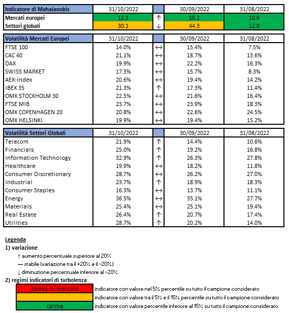
Gli indici utilizzati sono:

Le volatilità riportate sono storiche e calcolate sugli ultimi 30 trading days disponibili. Per ogni asset-class dunque sono prima calcolati i rendimenti logaritmici dei prezzi degli indici di riferimento, successivamente si procede col calcolo della deviazione standard dei rendimenti, ed infine si procede a moltiplicare la deviazione standard per il fattore di annualizzazione.
Per il calcolo della distanza di Mahalnobis si procede dapprima con la stima della matrice di covarianza tra le asset-class. Si considera l’approccio delle finestre mobili. Come con la volatilità, si procede prima con il calcolo dei rendimenti logaritmici e poi con la stima storica della matrice di covarianza, come riportato di seguito.
Supponendo una finestra mobile di T periodi, viene calcolato il valore medio e la matrice varianza covarianza al tempo t come segue:
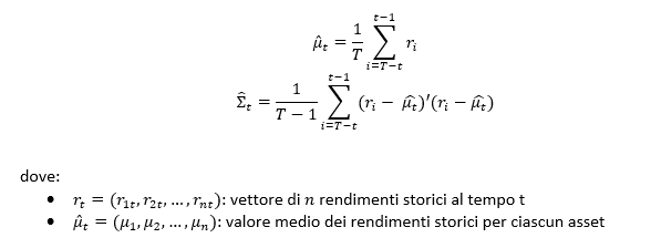
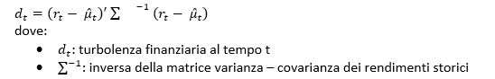
La distanza di Mahalanobis è definita formalmente come:
Le parametrizzazioni che sono state scelte sono:
Le statistiche percentili sono state calcolate a partire dalla distribuzione dell’indicatore di Mahalanobis dal Dicembre 1997 al Dicembre 2019 su rilevazioni mensili.
Ulteriori dettagli sono riportati in questo articolo.
Disclaimer: Le informazioni contenute in questa pagina sono esclusivamente a scopo informativo e per uso personale. Le informazioni possono essere modificate da finriskalert.it in qualsiasi momento e senza preavviso. Finriskalert.it non può fornire alcuna garanzia in merito all’affidabilità, completezza, esattezza ed attualità dei dati riportati e, pertanto, non assume alcuna responsabilità per qualsiasi danno legato all’uso, proprio o improprio delle informazioni contenute in questa pagina. I contenuti presenti in questa pagina non devono in alcun modo essere intesi come consigli finanziari, economici, giuridici, fiscali o di altra natura e nessuna decisione d’investimento o qualsiasi altra decisione deve essere presa unicamente sulla base di questi dati.

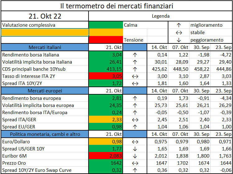
L’iniziativa di Finriskalert.it “Il termometro dei mercati finanziari” vuole presentare un indicatore settimanale sul grado di turbolenza/tensione dei mercati finanziari, con particolare attenzione all’Italia.
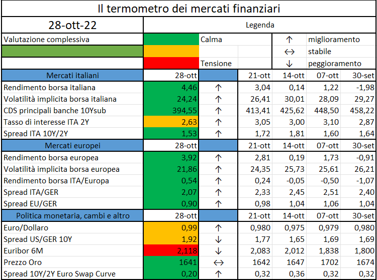
Significato degli indicatori
I colori sono assegnati in un’ottica VaR: se il valore riportato è superiore (inferiore) al quantile al 15%, il colore utilizzato è l’arancione. Se il valore riportato è superiore (inferiore) al quantile al 5% il colore utilizzato è il rosso. La banda (verso l’alto o verso il basso) viene selezionata, a seconda dell’indicatore, nella direzione dell’instabilità del mercato. I quantili vengono ricostruiti prendendo la serie storica di un anno di osservazioni: ad esempio, un valore in una casella rossa significa che appartiene al 5% dei valori meno positivi riscontrati nell’ultimo anno. Per le prime tre voci della sezione “Politica Monetaria”, le bande per definire il colore sono simmetriche (valori in positivo e in negativo). I dati riportati provengono dal database Thomson Reuters. Infine, la tendenza mostra la dinamica in atto e viene rappresentata dalle frecce: ↑,↓, ↔ indicano rispettivamente miglioramento, peggioramento, stabilità rispetto alla rilevazione precedente.
Disclaimer: Le informazioni contenute in questa pagina sono esclusivamente a scopo informativo e per uso personale. Le informazioni possono essere modificate da finriskalert.it in qualsiasi momento e senza preavviso. Finriskalert.it non può fornire alcuna garanzia in merito all’affidabilità, completezza, esattezza ed attualità dei dati riportati e, pertanto, non assume alcuna responsabilità per qualsiasi danno legato all’uso, proprio o improprio delle informazioni contenute in questa pagina. I contenuti presenti in questa pagina non devono in alcun modo essere intesi come consigli finanziari, economici, giuridici, fiscali o di altra natura e nessuna decisione d’investimento o qualsiasi altra decisione deve essere presa unicamente sulla base di questi dati.
The European Securities and Markets Authority (ESMA), the EU’s financial markets regulator and supervisor, is changing its Union Strategic Supervisory Priorities (USSPs) to include ESG disclosures alongside market data quality…
On 10 October 2022 the ECB announced the extension of the bilateral euro-renminbi currency swap arrangement between the ECB and the People’s Bank of China for another three years. The related press release is available on the ECB’s website…
https://www.ecb.europa.eu//press/govcdec/otherdec/2022/html/ecb.gc221028~b39a5a2227.en.html
Crypto may pose some risks to financial stability but may just need clearer guidelines rather than an entirely new set of rules, Christy Goldsmith Romero, a commissioner at the Commodity Futures Trading Commission, said…
Piero Cipollone, Vice Direttore Generale della Banca d’Italia, è intervenuto oggi al convegno “Le cripto attività: un terreno di nuove opportunità e sfide…

L’iniziativa di Finriskalert.it “Il termometro dei mercati finanziari” vuole presentare un indicatore settimanale sul grado di turbolenza/tensione dei mercati finanziari, con particolare attenzione all’Italia.
Significato degli indicatori
I colori sono assegnati in un’ottica VaR: se il valore riportato è superiore (inferiore) al quantile al 15%, il colore utilizzato è l’arancione. Se il valore riportato è superiore (inferiore) al quantile al 5% il colore utilizzato è il rosso. La banda (verso l’alto o verso il basso) viene selezionata, a seconda dell’indicatore, nella direzione dell’instabilità del mercato. I quantili vengono ricostruiti prendendo la serie storica di un anno di osservazioni: ad esempio, un valore in una casella rossa significa che appartiene al 5% dei valori meno positivi riscontrati nell’ultimo anno. Per le prime tre voci della sezione “Politica Monetaria”, le bande per definire il colore sono simmetriche (valori in positivo e in negativo). I dati riportati provengono dal database Thomson Reuters. Infine, la tendenza mostra la dinamica in atto e viene rappresentata dalle frecce: ↑,↓, ↔ indicano rispettivamente miglioramento, peggioramento, stabilità rispetto alla rilevazione precedente.
Disclaimer: Le informazioni contenute in questa pagina sono esclusivamente a scopo informativo e per uso personale. Le informazioni possono essere modificate da finriskalert.it in qualsiasi momento e senza preavviso. Finriskalert.it non può fornire alcuna garanzia in merito all’affidabilità, completezza, esattezza ed attualità dei dati riportati e, pertanto, non assume alcuna responsabilità per qualsiasi danno legato all’uso, proprio o improprio delle informazioni contenute in questa pagina. I contenuti presenti in questa pagina non devono in alcun modo essere intesi come consigli finanziari, economici, giuridici, fiscali o di altra natura e nessuna decisione d’investimento o qualsiasi altra decisione deve essere presa unicamente sulla base di questi dati.
