POSTPONED TO JUNE 10-11, 2021 DUE TO THE COVID-19 EMERGENCY
www.mate.polimi.it/fintech
Big Data and Machine Learning are driving
a significant transformation in the financial industry. Amazing examples
include: robo-advisory; predicting frauds in payment systems; development of sophisticated
algorithmic trading strategies; systemic risk assessment; rating of
companies/financial products using a huge amount of information; development of
chatbots for customers; nowcasting of financial time series; digital marketing;
instant pricing of insurance products.
The transformation concerns the
academia and the financial industry. The goal of the conference is to bring
together academicians with different backgrounds (economists, finance experts,
data scientists, econometricians) and representatives of the financial industry
(banks, asset management, insurance companies) working in this field.
Papers on all areas dealing with Machine
Learning and Big Data in finance (including Natural Language Processing and
Artificial Intelligence techniques) are welcomed. The conference targets papers
with different angles (methodological and applications to finance).
Invited speakers:
Tomaso Aste (University College London)
Emanuele Borgonovo (Università Bocconi)
Orlando Machado (Aviva Quantum)
Juri
Marcucci (Bank of Italy)
Georgios
Sermpinis (Adam Smith Business School, University of Glasgow)
Submission of the papers deadline: March 30th, 2021
Notification deadline: April 20th, 2021
Scientific
Committee:
Emilio Barucci (Politecnico di Milano, chair), Filippo Della Casa (UNIPOL), Paolo
Giudici (Università di Pavia), Daniele Marazzina (Politecnico di Milano), Andrea
Prampolini (Banca IMI), Marcello Restelli (Politecnico di Milano).
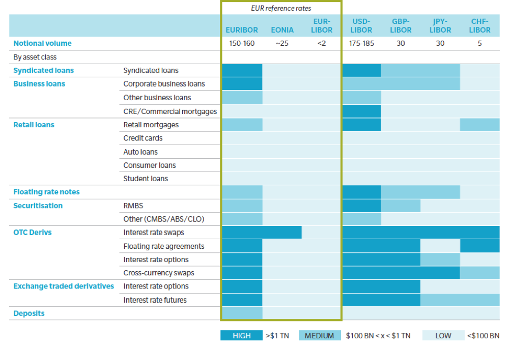
I tassi IBOR svolgono un ruolo fondamentale nei mercati
finanziari: in particolare il LIBOR è il tasso di interesse predominante per i
contratti (ad esempio interest rate swap, mutui, obbligazioni a tasso
variabile) nelle valute USD, GBP, CHF e JPY, mentre l’EURIBOR è il tasso più
diffuso per i contratti dell’area Euro (cfr. Figure 1).
A seguito della crisi finanziaria, tuttavia, la loro affidabilità e coerenza sono state messe in discussione per le acclarate manipolazioni e per il calo della liquidità del mercato interbancario. La crisi ha inoltre determinato una esplosione delle basi quotate fra tassi che differiscono per divisa o tenor, con conseguente moltiplicazione delle curve di tasso necessarie per valutare a mercato gli strumenti finanziari, e la necessità di gestire il corrispondente basis risk [1]. Tali basi sono la conseguenza del meccanismo di fixing dei tassi, riferiti a depositi interbancari a termine unsecured, e riflettono essenzialmente il rischio di credito e liquidità delle banche partecipanti (IBOR panel banks).
A partire dal 2009, le autorità e gli operatori del mercato hanno
intrapreso una serie di iniziative per rinnovare la governance dei principali
tassi d’interesse di riferimento e per individuare nuovi tassi basati su
transazioni reali in mercati di riferimento stabili e liquidi. In particolare,
i “Principles for Financial Benchmarks” emanati da IOSCO nel 2013 stabiliscono
4 aspetti principali per la determinazione dei tassi benchmark: Governance,
Quality of Benchmark, Quality of Methodology ed Accountability. Tali principi
sono stati accolti nell’area Euro dalla Benchmark Regulation (BMR), che
dichiara i tassi EURIBOR ed EONIA come “critical benchmark” ed impone quindi,
entro due anni dall’entrata in vigore (ovvero entro il 1 gennaio 2020), una
loro revisione per renderli aderenti oppure una loro sostituzione.
Il Financial Stability Board (FSB) ha raccomandato di rafforzare
tali tassi di interesse, ancorandoli a transazioni osservabili, consigliando lo
sviluppo di nuovi tassi risk free (RFR). A questo fine sono stati predisposti
cinque Working Group per le principali valute, che hanno individuato i
rispettivi RFR alternativi: in tutti i casi si tratta di tassi overnight
(secured per alcune divise ovvero unsecured per altre). Per la divisa USD è
stato scelto il tasso SOFR (Secured Overnight Financing Rate), mentre per EUR è
praticamente definito il nuovo tasso ESTER (Euro Short Term Rate, unsecured). I
tassi overnight, specialmente secured, non sono strettamente tassi privi di
rischio, ma possono essere considerati come buone approssimazioni in tal senso.
Nel luglio 2018 AFME, ICMA, ISDA, SIFMA e SIFMA AMG hanno
pubblicato l’esito della consultazione rivolta agli operatori di mercato, nella
quale vengono identificati i punti di attenzione della riforma dell’IBOR e le
raccomandazioni sugli step da effettuare per prepararsi al passaggio ai nuovi
RFR e dalla quale è emerso che esistono carenze sostanziali circa la
consapevolezza della tematica e gli step finora intrapresi per gestire la
transizione.
Transizione
I nuovi contratti conclusi dopo la scadenza BMR (1° gennaio 2020)
dovranno essere riferiti ai nuovi RFR. I contratti pre-esistenti (legacy
contracts) potranno essere re-indicizzati ai nuovi RFR oppure, se continueranno
ad essere pubblicati, contare ancora sui vecchi tassi IBOR. In entrambi i casi
sarà necessaria una modalità di transizione (“fallback”) verso i nuovi RFR.
Un passaggio molto importante in tale transizione sarà la
costruzione di una struttura a termine per i tassi RFR, sostitutiva
dell’analoga struttura a termine oggi quotata per i tassi IBOR sotto forma di
tassi di deposito, Futures, FRA (Forward Rate Agreement), e Swap. I nuovi RFR,
non disponendo di una struttura a termine con diverse scadenze, richiedono la
definizione di una regola per costruire dei tassi a termine. Ad esempio il
tasso a 3 mesi può essere costruito come composizione semplice dei tassi overnight
sul periodo. Questo tipo di indicizzazione è già ad oggi utilizzata per gli
strumenti di tipo OIS (Overnight Indexed Swap) scambiati sul mercato OTC. Sarà
poi necessario lo sviluppo di un mercato OTC liquido per tali strumenti
finanziari.
L’ISDA ha avviato un’iniziativa a livello internazionale per
identificare regole di fallback condivise per gli strumenti derivati, le quali
entreranno in vigore nel momento dell’interruzione permanente nella
contribuzione degli attuali benchmark. La soluzione di fallback si basa
sull’individuazione di un term adjustment e di uno spread adjustment da
applicare al RFR individuato. A luglio 2018, l’ISDA ha lanciato una prima
consultazione con la proposta di 4 metodologie alternative per il calcolo del
term adjustment e 3 metodologie per il calcolo dello spread adjustment, per le
divise GBP, CHF, JPY, i cui risultati sono attesi entro dicembre 2018. Una
successiva consultazione verrà lanciata per USD ed EUR nel 2019.
Tale metodologia, una volta definita e condivisa, sarà tuttavia applicabile per i soli derivati stipulati sotto ISDA agreement, mentre per gli altri strumenti (e.g. derivati non-ISDA, mutui, titoli) la conversione dovrà essere stabilita e non necessariamente avrà luogo con metodi analoghi, con il rischio di far emergere possibili basis mismatch e conseguenti conflitti contrattuali.
Area Euro
La normativa BMR ha sancito la fine dei tassi EONIA ed EURIBOR
così come li conosciamo. L’European Money Markets Institute (EMMI),
amministratore di entrambi i tassi, sta effettuando una revisione delle
metodologie attuali.
Per quanto riguarda l’EONIA, dopo una fase di studio, l’EMMI ha
ritenuto che la liquidità di mercato alla base del meccanismo di formazione
dell’EONIA non sia sufficiente per renderlo conforme alla BMR, e si è resa
quindi necessaria l’identificazione di un nuovo RFR in sua sostituzione. A tal
proposito l’European Central Bank (ECB) ha instituito il Working Group
sull’Euro Risk Free Rate, che il 13 settembre 2018 ha suggerito l’ESTER
(European Short Term Rate) quale nuovo RFR per l’Euro. Mentre l’EONIA è un
tasso di lending basato su depositi interbancari overnight effettuati sulla
piattaforma Real Time Gross Settlement (RTGS) operata dall’ECB, ESTER è un
tasso borrowing basato delle transazioni riportate dalle banche tramite il
Money Market Statistical Reporting (MMSR), e viene calcolato come media
ponderata sui volumi superiori al milione di euro, escludendo il primo 25% e
l’ultimo 25% della distribuzione dei tassi. L’ESTER, sviluppato dall’ECB
stessa, sarà ufficialmente pubblicato a partire da ottobre 2019; nel frattempo,
viene pubblicato un tasso pre-ESTER (osservazioni giornaliere a partire dal
marzo 2017 con la medesima metodologia di calcolo utilizzata a tendere) allo
scopo di familiarizzare con il nuovo tasso. I dati finora pubblicati dimostrano
che pre-ESTER è inferiore all’EONIA di circa 8-9 bps e maggiormente stabile
(minore volatilità storica e minori spike).
Per quanto riguarda l’EURIBOR, EMMI ha definito una metodologia
ibrida, attualmente in consultazione, che mira a superare le problematiche
dell’attuale metodologia di calcolo con lo scopo di ottenere un tasso che
minimizzi le possibilità di manipolazione e risulti ancorato a transazioni
osservabili e resistente agli stress del mercato. Nel caso in cui tale
metodologia venisse accettata dai regolatori come aderente ai principi IOSCO e
la BMR (scadenza 1° gennaio 2020), il nuovo EURIBOR potrebbe presumibilmente
essere il naturale successore dell’EURIBOR attuale. Nel caso in cui, invece,
l’EURIBOR subisse la medesima sorte del LIBOR, anche l’area Euro si troverà ad
affrontare le medesime problematiche delle altre principali divise. Al
riguardo, nello stesso documento in cui veniva sancita la scelta dell’ESTER
come nuova tasso risk free, il Working Group sull’Euro RFR ha suggerito di
utilizzare l’ESTER come base di partenza per costruire un nuovo tasso benchmark
in sostituzione dell’EURIBOR.
Impatti
A seguito della riforma, che avrà un impatto trasversale a tutti i
mercati, le aree in cui si possono individuate gli effetti più importanti
riguardano la liquidità degli strumenti di mercato indicizzati ai nuovi tassi,
la costruzione di nuove curve di tasso e superfici di volatilità, la modifica
delle metodologie di pricing, delle coperture, e il calcolo dei rischi. Saranno
inoltre di primaria importanza gli aspetti legali, con una possibile revisione
di tutti i contratti indicizzati ai tassi oggetto di transizione, e la gestione
della clientela per gestire possibili effetti di mismatching e di litigation.
Inoltre, si porrà la necessità di effettuare modifiche ai processi aziendali ed
alle infrastrutture IT. Al riguardo, sarà necessario porre molta attenzione
sulla governance complessiva del processo di transizione, al fine di assicurare
la coerenza tra gli impatti dei cambiamenti imposti dalla riforma e di gestire
i relativi rischi.
In particolare, per quanto riguarda i rischi di mercato, si posso
identificare i seguenti temi più rilevanti.
Contribuzioni tassi benchmark: le banche coinvolte nella contribuzione dei tassi benchmark dovranno gestire la transizione verso la contribuzione dei nuovi tassi secondo le nuove regole stabilite dagli organismi di riferimento (ECB per ESTER e prevedibilmente EMMI per EURIBOR per l’area Euro).
Dati di mercato: andrà gestita la transizione verso i nuovi tassi benchmark utilizzati come fixing per la valutazione dei contratti ed i relativi strumenti di mercato indicizzati a tali tassi. Andranno inoltre gestite le corrispondenti serie storiche per finalità di risk management (cfr. oltre).
Curve e volatilità tasso: utilizzando i nuovi strumenti di mercato indicizzati ai nuovi tassi benchmark, andranno inoltre costruite le curve di tasso e superfici di volatilità, gestendo i probabili problemi di liquidità nel caso in cui il mercato dei nuovi derivati indicizzati a RFR non sia abbastanza liquido e/o i dati non presentino una appropriata granularità. Inoltre è prevedibile un periodo di transizione in cui sarà necessario mantenere sia le vecchie curve e volatilità IBOR-based che le nuove curve e volatilità basate sui nuovi RFR.
Collateral management: in caso di revisione dei tassi di interesse utilizzati per la remunerazione del collaterale, andrà gestita la transizione verso i nuovi tassi di marginazione con conseguente revisione di tutti gli accordi di collateralizzazione.
Metodologie di pricing: le revisioni di dati di mercato, curve e volatilità tasso ed accordi di collaterale porterà probabilmente ad una conseguente revisione delle metodologie di pricing degli strumenti finanziari, che si articolano sotto vari aspetti come segue.
La revisione dei tassi di remunerazione del collaterale implicherà un adeguamento delle curve di scontro utilizzate per l’attualizzazione dei flussi futuri, con conseguenti impatti di sensitivity e P&L.
Un ulteriore impatto può determinarsi negli aggiustamenti valutativi, in particolare nelle misure di credit/debt/funding value adjustment (CVA/DVA/FVA) relative alle operazioni non soggette a collateralizzazione, dovuto all’impatto sulle esposizioni future e allo spread di finanziamento.
Possibili fasi di illiquidità e di passaggio di curve e volatilità tasso potranno determinare problemi di calibrazione dei modelli di pricing e conseguenti instabilità di prezzi, sensitivity e P&L.
In caso di dismissione dei tassi IBOR in favore di tassi risk free si avrà una semplificazione nel numero delle curve e volatilità di tasso necessarie per valutare gli strumenti, ed una semplificazione delle corrispondenti sensitivity (delta e vega in particolare). Di conseguenza si potrà determinare anche una semplificazione dei modelli di pricing, con un ritorno di fatto al mondo mono-curva risalente al periodo pre-crisi 2007.
Scenari storici: le nuove curve e volatilità tasso potrebbero non avere, dapprincipio, sufficiente profondità storica per costruire degli scenari storici, con conseguente impatto sulle metriche di rischio che si basano sui dati di mercato storici (e.g. historical VaR).
Trading vs Banking Book: date le diverse composizioni e metriche di rischio, si avranno impatti diversi: in particolare, per il Trading Book si rileverà un impatto su VaR, sensitivity, CCR e CVA, mentre per il Banking Book la transizione avrà effetti sulle masse di Bond, Loan e altri strumenti di cartolarizzazione, sia in termini di liquidità che in termini di rischio di tasso di interesse.
Basis risk: nel caso in cui l’adozione dei nuovi RFR avvenga a velocità diverse, ad es. più velocemente per i derivati e più lentamente per gli strumenti cash, anche in funzione della divisa, sarà necessario gestire una situazione ibrida con diverse asset class esposte a diversi tassi ed il conseguente rischio base.
Impatti sul capitale: la transizione verso i nuovi tassi benchmark richiederà l’identificazione dei possibili impatti sulle metriche di assorbimento di capitale; ad esempio, la mancanza di dati storici sui nuovi RFR potrebbe avere degli impatti alla luce della nuova regolamentazione per il Trading Book (FRTB), dove un punto cruciale per il calcolo delle metriche è la distinzione fra “modellable” e “non-modellable risk factors”.
Modelli Interni di Rischio: le eventuali variazioni di modello andranno gestite nell’ambito delle regole vigenti per i modelli interni (cfr. EBA RTS 2016/07 e manuale TRIM).
Figure 1: Notional outstanding balances by reference rate, order of magnitude US$ Trillion as of Dec 2017. Source: Oliver Wyman, Jun.2018
Note
[1] Ad esempio, per gestire i derivati di tasso in divisa EUR il mercato utilizza 5 curve (OIS, EURIBOR 1M, 3M, 6M, 12M) e almeno 6 superfici di volatilità (Cap/Floor EURIBOR 1M, 3M, 6M, 12M, Swaption EURIBOR 3M, 6M). Molte altre curve sono necessarie per gestire derivati e/o collateral cross currency.
L’iniziativa di Finriskalert.it “Il termometro dei mercati finanziari” vuole presentare un indicatore settimanale sul grado di turbolenza/tensione dei mercati finanziari, con particolare attenzione all’Italia.
Rendimento borsa italiana: rendimento settimanale dell’indice della borsa italiana FTSEMIB;
Volatilità implicita borsa italiana: volatilità implicita calcolata considerando le opzioni at-the-money sul FTSEMIB a 3 mesi;
Future borsa italiana: valore del future sul FTSEMIB;
CDS principali banche 10Ysub: CDS medio delle obbligazioni subordinate a 10 anni delle principali banche italiane (Unicredit, Intesa San Paolo, MPS, Banco BPM);
Tasso di interesse ITA 2Y: tasso di interesse costruito sulla curva dei BTP con scadenza a due anni;
Spread ITA 10Y/2Y : differenza del tasso di interesse dei BTP a 10 anni e a 2 anni;
Rendimento borsa europea: rendimento settimanale dell’indice delle borse europee Eurostoxx;
Volatilità implicita borsa europea: volatilità implicita calcolata sulle opzioni at-the-money sull’indice Eurostoxx a scadenza 3 mesi;
Rendimento borsa ITA/Europa: differenza tra il rendimento settimanale della borsa italiana e quello delle borse europee, calcolato sugli indici FTSEMIB e Eurostoxx;
Spread ITA/GER: differenza tra i tassi di interesse italiani e tedeschi a 10 anni;
Spread EU/GER: differenza media tra i tassi di interesse dei principali paesi europei (Francia, Belgio, Spagna, Italia, Olanda) e quelli tedeschi a 10 anni;
Euro/dollaro: tasso di cambio euro/dollaro;
Spread US/GER 10Y: spread tra i tassi di interesse degli Stati Uniti e quelli tedeschi con scadenza 10 anni;
Prezzo Oro: quotazione dell’oro (in USD)
Euribor 6M: tasso euribor a 6 mesi.
Spread 10Y/2Y Euro Swap Curve: differenza del tasso della curva EURO ZONE IRS 3M a 10Y e 2Y;
I colori sono assegnati in un’ottica VaR: se il valore riportato è superiore (inferiore) al quantile al 15%, il colore utilizzato è l’arancione. Se il valore riportato è superiore (inferiore) al quantile al 5% il colore utilizzato è il rosso. La banda (verso l’alto o verso il basso) viene selezionata, a seconda dell’indicatore, nella direzione dell’instabilità del mercato. I quantili vengono ricostruiti prendendo la serie storica di un anno di osservazioni: ad esempio, un valore in una casella rossa significa che appartiene al 5% dei valori meno positivi riscontrati nell’ultimo anno. Per le prime tre voci della sezione “Politica Monetaria”, le bande per definire il colore sono simmetriche (valori in positivo e in negativo). I dati riportati provengono dal database Thomson Reuters. Infine, la tendenza mostra la dinamica in atto e viene rappresentata dalle frecce: ↑,↓, ↔ indicano rispettivamente miglioramento, peggioramento, stabilità rispetto alla rilevazione precedente.
A surge in staking demand has flipped Ethereum’s validator queues, easing fears of a mass sell-off and reinforcing confidence in long-term ETH staking.
Introductory statement by Piero Cipollone, Member of the Executive Board of the ECB, at the Committee on Economic and Monetary Affairs of the European Parliament
The U.S. jobs report revealed only 22,000 job additions in August, far below expectations, increasing the likelihood of a Fed rate cut. Still, BTC remains below $112K.
Andavo bel bello sull’alzaia del naviglio grande, come è mia abitudine, ripensando – tutto immerso nei miei pensieri – al noto incipit di Orazio[1], quando mi vedo Mario che mi saluta vistosamente, avendomi riconosciuto in bici nonostante il caschetto. Era seduto in un tavolino di quel bar che si trova dove il naviglio si biforca verso Bereguardo, all’altezza di Abbiategrasso, con tavolini e sedie che ricordano un periodo pre-rivoluzione industriale. Mostrava di godersi beato quel caldo pomeriggio assolato; mai avresti detto di essere ancora a fine febbraio in piena pianura padana.
“Ma tu cosa ci fai qui?” mi viene spontaneo chiedergli.
“A Bob, come resistere con una giornata così, da pieno Climate change! Saranno armeno 25 gradi“, afferma solare.
Nonostante il quarto di secolo milanese, le origini romane di Mario affioravano qua e là, in una parlata oramai quasi senza accento, anche chiamandomi con un soprannome che quasi nessuno usava più. In pensione da neppure due anni, da “sempre” nel trading di bond di ogni specie e natura, dai governativi ai corporate, la sua pancetta – adesso evidente – non avrebbe mai fatto indovinare i suoi trascorsi. Miti e leggende narravano che avesse un pelo sullo stomaco, da misurare rigorosamente in kilometri, che da giovane fosse stato persino coinvolto nello squeeze di alcune aste di BOT, acquistando da solo quasi tutta l’asta, rivendendola – dopo ore – tramite broker compiacenti ad un prezzo folle, a banche consapevoli di non potere negare l’agognato titolo di stato alla propria clientela. E per questo disposte a pagare qualsiasi prezzo. Ma sono probabilmente leggende di quando il mercato era forse più semplice, costituito in prevalenza da BOT people.
“Tu piuttosto, continui a giocare con l’Energy Finance?” continua lui.
Carbon Allowance. E derivati: ma semplici forward, Futures e Pronti-contro-Termine
“Si adesso mi sono occupato di derivati su Carbon Allowance, quei contratti alla base del meccanismo di cap&trade per controllare le emissioni di C02” rispondo.
“Sempre diavolerie con derivati super-complessi, comprensibili solo a te e alla tua cricca?” riprende, consapevole di utilizzare un leitmotiv della carta stampata.
“No Mario, tutto relativamente elementare. In UE, tutte le aziende inquinanti devono consegnare alla fine di aprile una Carbon Allowance per ogni tonnellata di C02 emessa l’anno solare precedente; una Allowance ti permette (allow) di inquinare per una tonnellata di C02 e può essere scambiata su un mercato regolamentato. La strategia di trading su Allowance è una semplice strategia di carry trading”, gli rispondo.
“Un Pronti-contro-Termine, voi amate sempre utilizzare termini sofisticati” fa Mario, quasi polemico.
“Esattamente. Compri a pronti la Carbon Allowance e vendi a termine tramite il corrispondente Forward o Futures. Un Repurchase agreement o Repo come lo si chiama nel resto del mondo” aggiungo.
“Beh, a questo ci arrivo anch’io, non ci vuole certo un’arca di scienza. Ma piuttosto, quanto so’ i volumi scambiati?” mi domanda.
“Un mercato primario di 180 miliardi di Euro ogni anno, anche se i futures scambiano spesso 10 volte di più. Ebbene, si osserva un carry di più dell’1 percento, dall’inizio del 2013” affermo.
Un arbitraggio incredibile, che non dovrebbe essere possibile sul mercato
M: “Bob, non ti riconosco più: sei proprio diventato un accademico che vive nell’iperuranio dei suoi modellini. Si vede che 8 anni di trading non ti sono serviti proprio a niente! Mo’ te stanno a regalà 100 punti base di carry con un titolo emesso dall’Unione Europea. Un arbitraggio del genere non regge più di qualche secondo in un mercato liquido come quello, mica per anni! Magari pretenderesti che questo regalo lo facciano proprio a te?”
B: “Come darti torto. Quando l’ho visto, ti confesso che è stata la mia prima reazione. Ma la storia è più complicata…”
M: “So’ tutt’orecchi. Anche se la vedo difficile che me convinci” replica Mario.
B: “Immagina di essere Sofia Rossi, responsabile finanza di una grossa corporation che opera nel settore energetico e coinvolta nel processo di decarbonization. Immagina che si debba finanziare per un paio di billion (bn)…” riprendo.
M: “… e che magari si ritrova qualche bn di Allowance nello stato patrimoniale” afferma calandosi subito nel ruolo.
B: “Sofia può percorre due strade. Una è emettere una obbligazione pagando il costo di finanziamento dell’azienda; l’altra è quella di vendere un paio di bn di Allowance (a pronti) e riacquistarli alla scadenza di interesse (a termine).”
M: “E Sofia sceglierà la soluzione che gli costerà meno” aggiunge Mario, mostrando di aver colto subito il punto.
B: “Ti dico di più. Oltre il 40% delle Allowance sono offerte gratis a tutta una serie di aziende che la UE desidera tutelare. E queste Allowance sono date a fine febbraio dell’anno precedente quello in cui vanno consegnate”.
M: “Mi vuoi dire che se le ritrovano sul bilancio ben 14 mesi prima! Che bel regalo dalla UE. Ma con questi ammontari di Allowance a disposizione, queste aziende rischiano di coprire tutte le loro necessità in termini di Capex” dice Mario, incredulo.
B: “A volte, anche ben più del loro Capex. In ogni caso, le aziende hanno a disposizione una possibilità di finanziamento semplice ed immediata”
M: “Quindi Sofia, confronterà nel tempo lo spread su €STR dei Pronti contro Termine con lo Z-spread su €STR del corporate. [2] Che utilizzeranno per stabilire se risulta più conveniente emettere una obbligazione o entrare nel Repo con Carbon Allowance… ” afferma Mario, mostrando di aver ben compreso.
B: “E’ proprio l’analisi che abbiamo fatto con Michele e Pietro [1]. Il primo spread, quello del Repo lo puoi chiamare Carbon-spread o C-spread –una quantità comune a tutto il mercato delle Carbon Allowance-, ed il secondo è il classico spread di credito dell’azienda di Sofia. In particolare, ci siamo concentrati sui 12 maggiori inquinatori in termini di C02 nella UE, costruendo un indice che è una media dello Z-spread, che abbiamo chiamato Z-index.”
M: “E perché solo dodici?”
B: “A partire dal tredicesimo, le tonnellate di C02 emesse si riducono di un fattore 10 rispetto al primo della lista.”
La cointegrazione che si osserva
Mentre mi mostra sul suo cellulare la Figura del paper [1] che ha già scaricato, con una capacità tecnologica che certo non mi appartiene, Mario mi domanda “E magari, avete mostrato che le due serie storiche sono correlate?”
B: “Quasi. In questi studi si verifica che le due serie siano cointegrate, cioè che le variazioni prime siano linearmente dipendenti” cerco di spiegare.
M: “Una specie di correlazione dei rendimenti degli spread”
B: “In pratica è proprio questo. Inoltre, verifichiamo attraverso un Error-correction-model che ogni qual volta si verifica una deviazione c’è un ritorno alla media. Sempre statisticamente significativo, per l’intero periodo di analisi.”
M: “Magari vorresti anche utilizzare le strategie mean-reverting di cui tu eri un fan… senza stop-loss. Mi ricordo la lavata di capo che avevi ricevuto dal boss; mostragli il backtesting della strategia senza uno straccio di stop-loss!”
B: “Caro Mario, certo che è possibile includere le stop-loss quando si osserva un comportamento mean-reverting, basta disegnare la strategia in maniera ottimale. Lo abbiamo fatto con Tommaso Santagostino-Baldi di JPM, con risultati incredibili (cf. [2]).”
M: “Ma Tommaso non faceva il trader da Goldman?”
B: “Per la verità adesso è a Citi. Sai come succede. Questi giovani smart, sono sempre pronti a serfare alla ricerca di lidi migliori, finché trovano onde sempre più sfidanti…”
M: “Comunque, l’inefficienza del Repo –che mi hai mostrato– è proprio impressionante. Un punto percentuale è tantissimo. E il fatto che permanga nel tempo. Mi sembra assurdo che non venga risucchiata subito dal sistema finanziario. Come mai succede?” domanda Mario impietoso.
B: “Le banche operano in questo mercato solo come intermediari. Durante tutto il periodo di analisi l’assorbimento di capitale era pari al 60% del nozionale sia per le Allowance che per i suoi derivati. Con questi costi in termini di capitale di certo in pancia non si tengono niente, neppure se arriva come collateral in un Repo”
M: “Quindi, le criticità non sono nel mercato delle Allowance ma nel mercato dei Repo di Allowance”
B: “Hai centrato la questione. Perché diventi efficiente, occorre costituire un mercato Repo di Carbon Allowance che sia liquido. Se liquido diventa efficiente”.
M: “Ricordo Ban Ki-moon, l’allora segretario generale dell’ONU: <<There is no Plan B, because there is no Planet B>>. Lo aveva dichiarato nel 2014, quasi gridando a New York”.
B: “E la situazione da allora non è certo migliorata. La soglia di 1.5 gradi Celsius di riscaldamento globale verrà superata in una manciata d’anni, se non si interviene molto rapidamente. Ad oggi non esistono molte alternative concrete e realizzabili alle Carbon Allowance. Le Allowance costituiscono di fatto l’unico strumento realmente implementato per il contenimento delle emissioni di C02. E dai primi tentativi nel 2008 in UE sono trascorsi quasi 20 anni; non c’è quindi tempo per tentare di implementarne un altro.
Le Allowance sono uno strumento che utilizza un meccanismo di mercato; questo è assodato. Questo meccanismo deve essere reso efficiente. E non c’è tempo da perdere.”
Ma la BCE cosa c’entra?
M: “Rendere efficiente un mercato Repo, mi dici poco. Bisognerebbe renderlo molto liquido. Solo con la BCE. Mi ricordo durante la Great Financial Crisis. Ti rammenti? Dopo Lehman, non si trovava quasi niente in Repo, neppure GC.[3] Solo quando la BCE ha esteso i panieri di bond ammessi nelle Repo operations in banca centrale, il mercato Repo ripartì. E molto rapidamente.”
B: “Basterebbe includere le Carbon Allowance, come collateral ammesso nelle Repo operations della BCE.”
M: “Bob, sei sempre il solito. Sembri uno di quei blogger economici da strapazzo. Mi meravigli: non riesci a tenere a mente neppure le basi. La BCE ha uno solo mandato: price stability, ovvero mantenere l’inflazione a medio termine nell’area dell’euro al 2%. Non si occupa mica di Climate Change e Carbon Allowance!”
B: “Quanto avviene sul clima ha un impatto significativo sull’inflazione. E le conseguenze possono essere devastanti.
Di sicuro l’impatto sull’inflazione dei cambiamenti climatici sarà molto più ampio di quello a due cifre osservato per la guerra in Ucraina, dove i timori di interruzioni di approvvigionamento si sono limitate a pochi prodotti agricoli (grano/mais e olio di semi), timori che in gran parte non si sono concretizzati. La supply chain europea è molto delicata: l’UE è importatrice netta di molti prodotti agricoli chiave, cruciali per il nostro approvvigionamento. Pensa, ad esempio, solo alla soia e derivati diretti, che influiscono sull’intera industria di trasformazione alimentare in quanto principale fonte di proteine per l’alimentazione degli animali dell’UE: più di 30 milioni di tonnellate all’anno, ovvero più di una dozzina di miliardi di euro all’anno. Quale sarebbe l’impatto secondo te in termini di inflazione se Argentina e Brasile, due dei tre principali fornitori della UE dovessero riscontrare problemi nella produzione dovuti al climate change? Che dici Mario, ti aspetti un’inflazione prossima al 2% in questo scenario?”, mi permetto di osservare.
M: “In effetti l’aumento di intensità e frequenza di eventi meteorologici estremi rendono questo tipo di eventi non più improbabili”, aggiunge Mario.
B: “Questo aumento sembra una conseguenza non solo del livello di concentrazione di CO2 in atmosfera, ma anche dalla sua derivata. La rapidità è stata incredibile: la concentrazione ha fatto registrare in pochi decenni cambiamenti pari a quelli osservati in centinaia di migliaia di anni, ammesso che questi livelli di C02 siano mai stati osservati dalla comparsa sulla faccia della terra delle prime scimmie antropomorfe…”.
M: “Mi hai convinto. Scusami se entro nel tecnico. Tuttavia la BCE accetta unicamente obbligazioni nelle 7 classi di bond ammessi come collateral; la volatilità delle Allowance sembrano molto maggiori di un bond governativo, forse più comparabile a quella delle azioni ”, replica.
B: “In effetti la volatilità delle Allowance non sono oggi molto diverse da quella di un indice azionario. Ti ricordo che la BCE accetta come collateral bond corporate decennali o anche trentennali! Credi forse che la volatilità di questi bond risulti inferiore?”
M: “No di certo, caro Bob. Rimane quindi solo una scelta di opportunità, però sarebbe una cosa mai vista. Secondo te quindi, la BCE potrebbe contribuire a salvare il pianeta!”
A un tratto si leva un intenso colpo di vento –improvviso– e trascina nelle acque del naviglio tavoli, sedie, tovaglie con corde aggrovigliate a cuscini e salviette. In piena val padana. Inaudito a fine febbraio. Mai visto.
“Mario, tutto bene?” gli domando.
Ma Mario, non risponde, non mi sente più. E’ rimasto seduto sulla sua sedia appoggiato sul suo tavolino, un tutt’uno rimasto completamente immobile come se nulla fosse successo. Lo vedo con gli occhi fissi sul cellulare a guardare diagrammi e schemi, o forse già a operare sul mercato… forse sussurra
[2] Baviera, Santagostino-Baldi (2019). Stop-loss and leverage in optimal statistical arbitrage with an application to energy market. Energy Economics, 79, 130-143. Disponibile su https://doi.org/10.1016/j.eneco.2018.03.024
[1] “Ìbam fòrte vià Sacrà, sicùt meus èst mos,/nèscio quìd meditàns nugàrum, tòtus in ìllis.” “Andavo bel bello per la via Sacra, come è mia abitudine,/ripensando – tutto immerso in quelle – a non so quali sciocchezze.” Quintus Horatius Flaccus (Orazio), Satira del sollecitatore, Sermones (Satire), I, 9 (30 a.c.). Traduzione dell’autore.
[2] L’Euro Short-Term Rate (€STR) è il tasso di interesse privo di rischio per l’area Euro, pubblicato dalla Banca Centrale Europea (BCE). Lo Z-spread è il classico spread che va aggiunto alla curva €STR per ottenere lo spread di credito dell’azienda dalle sue obbligazioni; la procedura stardard utilizzata sul mercato.
[3] General Collateral (GC), il mercato Repo più liquido, che generalmente coinvolge nell’area Euro bond governativi molto scambiati sul mercato.
[4] Pirandello, Luigi (1929). Enrico IV, conclusione della tragedia.
L’iniziativa di Finriskalert.it “Il termometro dei mercati finanziari” vuole presentare un indicatore settimanale sul grado di turbolenza/tensione dei mercati finanziari, con particolare attenzione all’Italia.
Rendimento borsa italiana: rendimento settimanale dell’indice della borsa italiana FTSEMIB;
Volatilità implicita borsa italiana: volatilità implicita calcolata considerando le opzioni at-the-money sul FTSEMIB a 3 mesi;
Future borsa italiana: valore del future sul FTSEMIB;
CDS principali banche 10Ysub: CDS medio delle obbligazioni subordinate a 10 anni delle principali banche italiane (Unicredit, Intesa San Paolo, MPS, Banco BPM);
Tasso di interesse ITA 2Y: tasso di interesse costruito sulla curva dei BTP con scadenza a due anni;
Spread ITA 10Y/2Y : differenza del tasso di interesse dei BTP a 10 anni e a 2 anni;
Rendimento borsa europea: rendimento settimanale dell’indice delle borse europee Eurostoxx;
Volatilità implicita borsa europea: volatilità implicita calcolata sulle opzioni at-the-money sull’indice Eurostoxx a scadenza 3 mesi;
Rendimento borsa ITA/Europa: differenza tra il rendimento settimanale della borsa italiana e quello delle borse europee, calcolato sugli indici FTSEMIB e Eurostoxx;
Spread ITA/GER: differenza tra i tassi di interesse italiani e tedeschi a 10 anni;
Spread EU/GER: differenza media tra i tassi di interesse dei principali paesi europei (Francia, Belgio, Spagna, Italia, Olanda) e quelli tedeschi a 10 anni;
Euro/dollaro: tasso di cambio euro/dollaro;
Spread US/GER 10Y: spread tra i tassi di interesse degli Stati Uniti e quelli tedeschi con scadenza 10 anni;
Prezzo Oro: quotazione dell’oro (in USD)
Euribor 6M: tasso euribor a 6 mesi.
Spread 10Y/2Y Euro Swap Curve: differenza del tasso della curva EURO ZONE IRS 3M a 10Y e 2Y;
I colori sono assegnati in un’ottica VaR: se il valore riportato è superiore (inferiore) al quantile al 15%, il colore utilizzato è l’arancione. Se il valore riportato è superiore (inferiore) al quantile al 5% il colore utilizzato è il rosso. La banda (verso l’alto o verso il basso) viene selezionata, a seconda dell’indicatore, nella direzione dell’instabilità del mercato. I quantili vengono ricostruiti prendendo la serie storica di un anno di osservazioni: ad esempio, un valore in una casella rossa significa che appartiene al 5% dei valori meno positivi riscontrati nell’ultimo anno. Per le prime tre voci della sezione “Politica Monetaria”, le bande per definire il colore sono simmetriche (valori in positivo e in negativo). I dati riportati provengono dal database Thomson Reuters. Infine, la tendenza mostra la dinamica in atto e viene rappresentata dalle frecce: ↑,↓, ↔ indicano rispettivamente miglioramento, peggioramento, stabilità rispetto alla rilevazione precedente.
A new report by Ripple and CB Insights reveals how banks are reshaping financial markets through digital asset infrastructure, tokenization and crypto partnerships.
The European Securities and Markets Authority (ESMA), the EU’s financial markets regulator and supervisor, has today published the new quarterly liquidity assessment of bonds.
Following the publishment of the draft Delegated Act [5] and concerned to the main items falling under Pillar I, this article explores the confirmation and changes to the “best guess” rules outlined in [4] and highlights the remaining areas of uncertainty. Technical discussions are complemented with numerical examples at 25Q2, together with impact assessments based on simplified insurance portfolios that cover several Macaulay liabilities durations (short 5y; medium 10y; long 15y) and duration gaps (-/+1.5y). The opinions expressed by the Author represent her view and do not necessarily represent the position or opinion of her employer.
The changes to the SII Directive [2] were published on the 08.01.25 in the Official Journal of the European Union by the European Parliament and European Council, with new measures expected to enter in force by the end of January 2027. On the 17.07.25 the European Commission published a proposal for the revision of the SII Delegated Act [5], opening a consultation phase that will last till the 05.09.25. The extension of the 4-weeks standard consultation period considers the summer holidays and aims at landing the final acts before year end, to help the market meeting the enter in force due date. Technical Standards are expected to come.
It is worth recalling that the revision of the SII directive twists together with the adoption of the Insurance Capital Standards (ICS) from the IAIS (International Association of Insurance Supervisors) [3]: the IAIS will begin developing a detailed ICS assessment methodology in 2025, monitoring the implementation process in 2026, with the aim of starting a detailed assessment of the ICS implementation in 2027.
Before Deeping dive into the details of the changes, it is worth recalling the aim the European Commission.
The insurance sector is a key institutional investor to contribute to the European Union priorities (defence, research, innovation and the green and digital transitions), with around 10 trillion of assets under management. In view of the long-term nature of its business, the insurance section is well-placed to provide stable funding to the real economy, including long-term capital financing to small-medium enterprises and small mid-caps, or investments in equity and certain alternative assets (such as venture capital, private equity and infrastructure). Insurers can also contribute to securitisation by facilitating the transfer of risks outside the banking sector. As of today, the share of the insurance sector in such investments is very limited. The amendments proposed in the draft delegated acts (such as those related to the risk margin calculation and the long-term equity investments) are aimed at increasing the capital in excess of the solvency capital requirement (SCR), strengthening the undertakings’ capacity to support the real economy of the European Union. The lower risk charges for the securitizations investments aim at facilitating the risk transfer outside the banking sector. Supervisory authorities are encouraged to monitor how the freed-up capital is being used, including its effect on insurers’ capital positions over time.
The main changes falling under Pillar I are:
interpolation and extrapolation of the base risk-free yield curve
determination of the volatility adjustment
calculation of the risk margin
interest rate risk sub-module: stresses definition and correlation parameters
equity risk sub-module: symmetric adjustments and qualifying criteria for long term equity investment
catastrophe risk (non-life catastrophe sub-module) and potential treatment of sustainability risk
capital requirements of securitisation positions
simplified calculations
dividends, risk-mitigation techniques and counterparty default risk
Points a) to f) were already covered in [4], while g) to i) are now being addressed. The numerical examples provided are based on 25Q2 market data and derived on simplified insurance portfolios whose cash flows are linearly decreasing over time and subject to the discount effect only: the liabilities are fully composed by minimum guarantees (i.e. no change assumed in the future discretionary benefits following movements in rates) and the backing assets, bonds-like, have the same market value as the liabilities in t=0, with the remaining assets defining the base own funds not subject to interest rates movements. The base own funds are assumed to be about 10% of the total assets.
Base risk-free yield curve
No changes compared to what the Author described in [4], a minor doubt remains on the VA application to the first element of the LLFR.
The formulas to extrapolate the risk free yield curve are outlined in the draft delegated acts, confirming the definition of the extrapolated forward rates being a weighted average between the last liquid forward rate (LLFR) and the ultimate forward rate (UFR), with speed of convergence to the UFR equal to a=11% for all the currency except for the Swedish Krona (a=40%).
For each year h exceeding the first smoothing point (FSP) the (continuous compounded) annual forward rate is defined as
and the extrapolated (annual compounded) spot rates are equal to
Note that
where (cc) and (ac) respectively indicate the continuous and annual compounding.
The FSP corresponds to a maturity for which the volume of outstanding bonds of that or longer maturities is sufficiently high. To confirm the First Smoothing Point (FSP) for EUR to be 20y at end January 2027, the currency related threshold is rounded up to 8%, including a safety margin, given the increase in long-maturity bonds observed in recent years.
The LLFR is defined as a weighted average of multi-years annualized continuously compounded forward rates. The first one covers a period prior to the FSP and the other periods starting at the FSP and lasting up to maturities where the swaps are available from DTL (deep, liquid and transparent) markets. The weights to apply to these multi-years annualized forward rates are derived by the average notional amount of traded contracts of interest rate swaps of the respective relevant maturities. Please refer to [4] for the best guess adopted in the calculations.
As commented in [4] the Author believes that this new definition of the base risk-free yield curve introduces discontinuities in the forward rates, by “patching” two pieces of information: one coming from the market data up to the FSP, and the other coming from the extrapolation.
It must be noted that the volatility adjustment is applied only to the first annualized continuously compounded forward rate of those summed up to define the LLFR and is therefore just partially accounted for in the extrapolation (by a share equal to the first weight). It is not yet clear whether the VA shall be translated into an equivalent continuous compound rate to be correctly summed up to a value expressed in continuous compounding.
A 5-year phasing-in mechanism may be applied, subject to approval, by linearly decreasing the speed of convergence a at the beginning of each calendar year from 20% during the year starting at 1st January 2027, to 11% on 1st January 2032 (Swedish Krona from 70% to 40%).
Volatility adjustment (VA)
Additional clarifications are provided compared to what the Author described in [4], but some areas of uncertainty remain.
The definition of the spread (S) to be adopted in the VA calculation is given, such as the parameters and formulas to use for the risk correction (RC) calculation. Additional specifications are provided for the calculation of the credit spread sensitivity ratio (CSSR).
Namely:
where
wgovt and wcorp denote the ratios of the value of respectively government bonds (govt) and bonds other than government, loans and securitisations (corp) compared to the value of all bonds, loans and securitizations included in the reference portfolio of assets for the currency or country under examination (i.e. the two sum up to 100%). Government bonds are meant to describe exposures to both central governments and central banks. These definitions clarify that that the reference portfolio adopted for the calculation of the macro component shall be the country reference portfolios provided by EIOPA, and not that of the undertakings.
sgovt and scorp denote the average currency spread of respectively government bonds and bonds other than government, loans and securitisations included in the reference portfolio of assets for the currency or country under examination
It is worth noting that the spread levels can go negative, while being floored to 0 in the current calculation. This may produce a lower VA, albeit being irrelevant in the current market situation and considering the duration of the assets in the reference portfolios.
The risk corrections (RC for both the govt and corp parts) are defined according to this formula and parameters
where
cap
pcI
pcII
pcIII
govt
65%
30%
20%
15%
corp
125%
50%
40%
35%
The parametrization chosen is the “Option 3” reported in [4]. LTAS is based on data relating to the last 30 years (or replaced by constructed data when not available) and x+ = max(0,x).
Note that
The formula for the credit spread sensitivity ratio is confirmed to be
where the two PVBP indicate the Price Value of a Basis Point of respectively the values of the investments in bonds, loans and securitizations (MVA) and of the Best Estimate Liabilities (BEL) of an undertaking. These two PVBP are calculated by comparing the stressed value of the quantity (under respectively a parallel shift in credit spreads and interest rates) to its base value and standardizing the difference by the stress level. The stress level are set to the VA*, that is the level of the permanent volatility adjustment under the assumption of a CSSR=100%.
For the calculation of the latter, the undertakings should consider the effect of future discretionary benefits (FDB, i.e. the profit sharing). For the calculation of the former, the undertakings should exclude fixed income investments which give rise to no or residual credit spreads. The Autor’s interpretation on this is that undertakings should exclude investments which are not credit sensitive from a market perspective (such as checking accounts) or assets linked to liabilities capable of absorbing the shocks (such as Unit Linked assets) but should include assets credit sensitive that are hedged with derivatives and whose net exposure to credit stress may not be relevant. Indeed, the Author’s interpretation is that credit derivatives are excluded from the CSSR numerator calculation (assets PVBP), coherently to the CIC codes proposed by EIOPA in their 2020 opinion [1]. The Author believes that BEL values should be net of reinsurance and include Unit Linked contracts: the former allows for a correct calculation, the latter for a coherency of treatment of Unit Linked business where the VA is applied. Specific to the German market, it is not clear whether Surplus Funds should be included or excluded from the FDB (and therefore the BEL) value.
As pointed out in [4] the Author believes such CSSR formulation may either slow the calculation process or introduce dependences on previous quarters data (undertakings need time to have their assets and liabilities portfolios ready at the evaluation date). Finally, while understanding the reasons driving the choice of a stress level comparable to the permanent VA (that correctly captures the convexity of the liabilities), the Author wonders if that could be substituted by a fixed parameters (like 25bps) that can be updated by EIOPA once a year. Indeed, having a stress value that varies in time may cause an undue effect: an undertaking whose portfolios (and so the credit and interest rate sensitivities) do not change over time should calculate the same PVPB(BEL) but may experience different outcomes driven by changes in VA*, just because of different stressing levels and interconnections with sampling errors of stochastic evaluations.
Risk Margin
A little change compared to what the Author described in [4] concerning the decay parameter.
The Risk Margin formula is amended to introduce an exponential term-dependent factor (λ=96%, compared to the 97.5% proposed by EIOPA in their 2020 opinion [1] and used as best guess by the Author in [4]), with decrease floored to 50%. This correction fixes the bias of the current definition, reducing the technical provisions and releasing capital, that is expected to be channelled towards productive investments in the real economy. The cos-of capital rate (CoC=4.75%) introduced by the Directive (EU) 2025/2 is confirmed. In the formula, z denotes the annual compounded zero risk free rate
The Author already pointed out in [4] the competitive disadvantage for European life insurers compared to UK peers (whose supervisor is the PRA – Prudential Regulation Authority), that are subject to a CoC=4%, λ=90% and floor=25%.
Compared to the current regulation, these amendments produce an important release in capital, almost halving the value of the RM for a 7y duration portfolio (with the decrease in RM being about -40% = (96%^7)*(4.75%/6.00%) – 1).
Interest Rates stresses and correlation
The main items described by the Author in [4] remains the same, with some changes in the stress parametrization, some clarifications provided around the convergency and few areas of uncertainty still pending. Indeed, the delegated acts amend the rules to allow for:
a lower correlation between the spread risk and interest rate risk in interest down scenario (decreased from 50% to 25%), that was examined by EIOPA in their 2020 review [1], but not quoted in the amendments to the SII Directive [2]
the need of extrapolate the stressed interest rates beyond the FSP, following the same methodology adopted for the base case and a stressed UFR (-/+15bps) and a stressed LLFR (where the rates at the maturities considered are stressed). The Author believes that stressing the LLFR is far too complicated compared to the benefits it may bring. Furthermore, for the EUR currency, the calculation would imply the need of stressing parameters for tenors (t=20, 25, 30, 40 and 50) after the FSP: are those published (designed for zero rates) suitable for “multi-year” forward rates hold constant between the illiquidity windows?
The extrapolation of the stressed yield curves causes an additional burden from a practical perspective and is also debatable from a theoretical perspective: one could claim that just a massive structural change in the economy would lead to a change in UFR, others may agree that it can move by -/+15bps, others may think it should move more. Back in 2018 (EIOPA’s second set of advice to the European Commission on specific items in the Solvency II Delegated Regulation), EIOPA hinted that the UFR in stressed scenarios could be higher than 15bps
the need to allow for interest rates to become negative, or to decrease further when they are already negative, including a maturity-dependent floor (that reflects the lower plausibility of extreme long-term rates, being equal to -1.25% up to 7 years, -0.893% after 20 years and linearly interpolated in-between)
the stress methodology that moves from relative shocks to a combination of relative and absolute shocks (derived from a relative displaced model)
where zt denote the risk free zero rates without VA and st and bt are defined for integer maturities t=1:50, then linearly interpolated to respectively 20% (st) and 0% (bt) between t=50 and t=90/60. For maturities shorter than a year, st and bt should be equal to those of maturity 1.
The Author believes that the rules to calculate the stressed parameters for maturities longer than 50 years are redundant, since stressed rates have to be extrapolated and the current maximum last liquid point (LLP) is 50y for the GBP currency
As shown in the following pictures, it is worth nothing that:
compared to the current, the alternative down shock is much harsher than the up one; the alternative up shock can even be less conservative than the current due to the in-force application of a floor (the up stress shall be at minimum 1%)
the new formulation succeeds the back testing exercise of replicating the 1y fall in rates occurred between 31.12.19 and 31.12.20 but fails at capturing the 1y spike occurred between 31.12.21 and 31.12.22
As a minor note, the proposed stressing parameters slightly deviate from those reported by EIOPA in their 2020 opinion [1] for maturities greater than 20y, that do not impact the results because of the extrapolation (or has a minor impact because of the stressed LLFR).
Finally, while the amendments to the Directive [2] quoted a not-so-clear approach to the phasing-in mechanism (“amendments to the interest rate risk sub-module may be phased in over a transitional period of up to five years. Such phasing-in shall be mandatory and apply to all insurance or reinsurance undertakings”), nothing is said in the draft delegated acts [5]. The Author believes that the phasing-in mechanism should not be mandatory: in case an undertaking was well matched, with negligible (or positive) impacts coming from the amendments in the regulation, the phasing in would become a disadvantage, adding an undue burden from a process perspective.
An impact assessment is performed on six simplified insurance portfolios to compare their loss in own funds (OF) under stress conditions: three liabilities durations are considered (short 5y, medium 10y and long 15y) as well as two duration gaps (-/+1.5y). As expected, portfolios with negative/positive duration gap (i.e. Liabilities longer/shorter than Assets) are exposed to the interest rate down/up risk. The table only shows the results of the portfolios where the scenario is biting, expressing their loss in OF (corresponding to the capital requirement of that scenario) in relative terms of the base OF value, like a capital charge metric.
short
medium
long
current
Irup
-22%
-22%
-19%
Irdown
-11%
-10%
-7%
revised
Irup
-33%
-21%
-11%
Irdown
-27%
-27%
-14%
In the IR down scenario, the revised capital charges are always higher than the current. In the IR up scenario, the revised capital charges are higher/comparable/lower than the current for portfolios with short/medium/long duration. In the latter the 1% minimum stress prevails that of the new formulation.
Equity risk sub-module: symmetric adjustments and qualifying criteria for long term equity investment
The symmetric adjustment boundaries are widened (not lower than -13% or higher than 13%, with limits increased from the current -/+10%), to generate greater variations in the standard equity capital charge, thereby enhancing its capacity to dampen the impact of sharp market fluctuations.
The other amendments aim at facilitating the insurers’ long-term investments in equity (subject to a reduced capital charge of 22% on the absolute value of the equity investments). They clarify the approach to demonstrate the undertakings’ ability to avoid force selling of such instruments, as well as the need of performing the assessment at the level of the funds (instead of their underlying assets) when holding investment funds. Finally, in article 173, the draft delegate acts introduce a new prudential treatment for equity investments that benefit from a significand subsidy or guarantee from public authorities (legislative programs), that can be qualified as long-term equity investments. These are subject to a limit: the standard equity risk submodule corresponding to such equity investments should not exceed 10% of the undertaking own funds. Concerning the force-selling assessment, article 171a clarifies that undertakings are allowed to select the most appropriate approach from several methods but cannot opportunistically switch between approaches over time (safeguards and supervisory monitoring requirements). Article 171d indicates that the assessment can be conducted at the level of the fund and that type 1 funds should be considered to present a lower risk profile for the purpose of identifying long-term equity investments, including when they are invested in qualifying infrastructure equities or qualifying infrastructure corporate equities.
Catastrophe risk and potential treatment of sustainability risk
The definition of perils (windstorm, earthquake, flood, hail, subsidence) in the scope of the natural cat sub-module are provided, together with some amendments on the parameters, risk weights and correlation coefficients for the calculation of the capital requirements; the man-made catastrophe risk module is simplified.
Undertakings shall put in place internal procedures to avoid overreliance on data from past events related to climate change trends and should include where appropriate the usage of climate scenarios. Moreover, article 297a of the draft delegated acts clarify that the solvency and financial condition report (SFCR) shall state whether the undertaking has any material exposure to climate change-related risks, following the materiality assessment, and, where relevant, whether it has taken any actions to manage such exposure.
Finally, the European Commission, together with EIOPA, will assess how sustainability risks related to fossil fuel assets and activities associated with high emissions are managed by insurance and reinsurance undertakings. The Commission will also consider, as part of the forthcoming European Climate Adaptation Plan, a mandate on whether prudential rules can be more conducive to issuances of or investments in catastrophe bonds and other green bonds.
Securitization positions
As institutional investors, insurance and reinsurance undertakings should be fully integrated into the Union’s securitisation market. STS (simple, transparent and standardized) instruments are securitizations that meet these criteria:
Simple: clear structure, free of complex derivatives or excessive layers
Transparent: extensive availability of data on the underlying pool and performance
Standardized: uniform rules for loan selection, monitoring, and investor protection
The draft delegate acts further align the risk factors for senior tranches of STS with those applicable to corporate or covered bonds, improving the consistency across asset classes with comparable risk profiles. Lower risk factors are introduced for senior tranches of non-STS securitizations to capture their high quality. Both changes significantly lower the risk charges compared to the current values. As an illustrative example, on a AAA STS senior with 2y of duration, the capital charge moves from 2.0% to 1.4%. The longer the duration, the higher the benefit (e.g. for 6y duration the capital charge moves from 5.60% to 4.00%). Similarly, for the AAA non-senior STS, the capital charge moves from 5.60% to 4.00% (2y duration) and from 15.60% to 10.90% (6y duration 6). The worse the rating, the higher the capital release. Securitizations becomes cheaper than comparable investment grade bonds.
Simplified calculations
Simplifications concern a carve-out from the mandatory application of the ‘look-through’ (LT) in investment funds (namely, the calculation of capital requirements based on each of the underlying assets of such funds) and exceptions to the use of external ratings.
Article 89a introduces the definition of a simplified formula to calculate the SCR of immaterial risk modules or sub-modules (other than the market risk and its sub-modules). This simplification can be adopted for three years from the reference date of calculation and is based on the undertaking’s specific volume measure for the risk.
Dividends, risk-mitigation techniques and counterparty default risk
Rules governing the calculation of foreseeable dividends are introduced (New Article 70a) to improve the level playing field: during the financial year, these should be deducted from the available own funds (OF) following an accrual approach, rather being immediately fully deducted. Dividends are foreseeable just if the person or body running the undertaking has formally taken a decision regarding the amount of dividend to be paid out (dividends normally corresponds to profits of the previous financial years).
Risk transfers between insurance and reinsurance sectors are facilitated in paragraph (18) (New Article 212a) by some forms of non-proportional reinsurance arrangements. These are called “adverse developments covers” and are explicitly recognized in the standard formula, where their risk mitigating effect is better reflected in the capital requirements.
Concerning the counterparty default risk module:
article 192 corrects the loss-given default formula for reinsurance contracts subject to collateral agreement, where =60% counterparty assets subject to collateral
rewarding the risk mitigating effect (change in sign) and modifying F from F to F’’’, that appears to still be 100%.
a floor to the loss-given defaults is introduced for the mortgage loans, to avoid unduly assumptions of these being risk-free (the standard formula capital requirement is currently null when the loan-to-value does not exceed 60%)
where Guarantee denotes the amount the guarantor would pay to the undertaking in case of default of the mortgage loan at the time when the value of the property held as a mortgage was equal to the 80% of the risk-adjusted value of the mortgage (Mortgage)
This new formulation replaces the current formula with 0 floor and 0 guarantee
similarly, the loss given default for defaulted loans or forborne loans is defined as
the rules governing the capital requirements on direct exposures to central clearing counterparties (CCPs) are amended to lower their counterparty default risk and make it comparable to that of indirect exposures
repurchase and securities landing/borrowing transactions are classified as type 1 exposures and the risk-reducing effect of central clearing (contractual netting) is recognized to improve the consistency with the treatment of derivatives and avoid an overly conservative capital requirement
where Exposure denotes the value of securities or cash lent to the counterparty under the transaction and Collateral denoted the risk-adjusted value od securities or cash received from the counterparty.
Lastly, the amounts expressed in euro in the current Delegated Regulation (2015/35) should be revised and inflated with a cumulative inflation that is approaching 35% since the entry in force of the regulation in 2014.
References
[1] “Opinion on the 2020 review of Solvency II” – EIOPA – 17.12.20
[2] “Directive (EU) 2025/2 of the European Parliament and of the Council amending Directive 2009/138/EC as regards … and amending Directives 2002/87/EC and 2013/34/EU” – European Parliament and European Council – 27.11.24
Questo sito utilizza cookie tecnici e di profilazione, propri e di terze parti, per garantire la corretta navigazione, analizzare il traffico e misurare l'efficacia delle attività di comunicazione.
Questo sito Web utilizza i cookie per migliorarne l'esperienza di navigazione. I cookie classificati come necessari, sono essenziali alle funzioni di base sito e vengono sempre memorizzati nel tuo browser. I cookie di terze parti, che ci aiutano ad analizzare e capire come utilizzi questo sito, vengono memorizzati nel tuo browser solo con il tuo consenso. Di seguito hai la possibilità di disattivare questi cookie. Tieni in conto che la disattivazione di alcuni di questi cookie potrebbe influire sulla tua esperienza di navigazione.
Necessary cookies are absolutely essential for the website to function properly. These cookies ensure basic functionalities and security features of the website, anonymously.
Cookie
Durata
Descrizione
cookielawinfo-checkbox-analytics
1 year
Cookie tecnico impostato dal plugin GDPR Cookie Consent che viene utilizzato per registrare il consenso dell'utente per i cookie nella categoria "Analitici".
cookielawinfo-checkbox-necessary
1 year
Cookie tecnico impostato dal plugin GDPR Cookie Consent che viene utilizzato per registrare il consenso dell'utente ai cookie.
CookieLawInfoConsent
1 year
Cookie tecnico impostato dal plugin GDPR Cookie Consent per salvare le scelte si/no dell'utente per ciascuna categoria.
viewed_cookie_policy
1 year
Cookie tecnico impostato dal plugin GDPR Cookie Consent che registra lo stato del pulsante predefinito della categoria corrispondente.
Analytical cookies are used to understand how visitors interact with the website. These cookies help provide information on metrics the number of visitors, bounce rate, traffic source, etc.
Cookie
Durata
Descrizione
_pk_id.gV3j99y0AE.0928
1 year 27 days
Cookie analitico impostato da Matomo e utilizzato per memorizzare alcuni dettagli sull'utente come l'ID univoco del visitatore
_pk_ses.gV3j99y0AE.0928
30 minutes
Cookie analitico impostato da Matomo di breve durata e utilizzato per memorizzare temporaneamente i dati della visita