Last 11 February 2019 the European Commission (EC) asked the European Insurance and Occupational Pension Authority (EIOPA) for a call for advice on the 2020 review of SII. As a response to that, EIOPA launched a public Consultation Paper (CP) on the 15^th October 2019 whose feedback were to be submitted by the 15^th January 2020 (Insurance and Reinsurance undertakings submitted their results to the NSAs last 6 December 2019, and the NSAs reported them to EIOPA last 8 January 2020). EIOPA is now collecting the data and assessing the impacts of its proposals, setting out the final advice by next 30^th June 2020. The proposals presented are a view of EIOPA and may not be adopted: the EC will balance political considerations to the technical ones. It’s interesting to notice that EIOPA has reiterated in the CP its suggestion of introducing negative interest rates in the SF SCR calculation (advice dated 2018) previously rejected by the EC.

The call for advice comprised 19 topics, which can be broadly divided into three parts

• review of the Long Term Guarantee (LTG) measures, always foreseen as being reviewed in 2020, as specified in the Omnibus II Directive
• potential introduction of new regulatory tools in the SII Directive, notably on macro-prudential issues, recovery and resolution, and insurance guarantee schemes
• revisions to the existing SII framework, including reporting and disclosure of the SCR.

The main proposals set out in the CP and discussed in the following are:

• choose a later Last Liquid Point (LLP) for the extrapolation of risk-free interest rates for the Euro or change the extrapolation method to take into account market information beyond that point; these are expected to increase both TP and SCR, particularly for firms with long duration businesses
• change the calculation of the Volatility Adjustment (VA), to address overshooting effects and to reflect the illiquidity of insurance liabilities; 8 variations are proposed and, albeit they may help in reducing the volatility caused by the current design, they may increase the complexity of the calculation and even reduce the overall protection provided by this measure
• review the calibration of the interest rate risk sub-module in line with empirical evidence, considering negative interest rates; this is expected to increase the SCR
• include macro-prudential tools in the SII Directive and establish a minimum harmonised recovery and resolution framework for insurance.

No changes have been proposed for the Risk Margin (RM), causing the disappointment of many firms that consider this metric too big for the annuity business and too sensitive to interest rates changes – and therefore sensitive to the changes proposed to the LLP.

Positive and negative proposals have been made with respect to the Matching Adjustment (MA), currently only applied in Spain and UK. A good aspect is that EIOPA has proposed to recognize diversification between MA and non-MA portfolios, reducing the SCR, but without showing any intention to make the MA more flexible and adding a further requirement on restructured assets that may make it harder for the firms to apply the MA.

Regarding [A], EIOPA has proposed 5 options to amend the Euro LLP:

1. no changes (i.e. LLP=20 years, Smith-Wilson extrapolation)
2. LLP=20 + safeguards in terms of disclosure and governance

sensitivity analysis on LLP=50 to be include in the RSR and SFCR; if the firms breach the SCR or MCR in the sensitivity analysis, they have to provide evidences that the policy holders protection is not put at stake by dividend payments and capital distributions, which can be limited by the NSAs in case the evidences were not satisfying

• LLP=30 + safeguards in terms of disclosure and governance (as in option 2)
• LLP=50
• alternative extrapolation method to consider market data beyond the LLP for all the currencies

Beyond causing a detriment to the SCR position of the insurance firms, options from 2 to 4 are quite onerous.

Regarding [B], EIOPA has proposed a reform to the VA calculation that comprises 8 different design options, 3 different General Application Ratio (GAR), the usage of Dynamic VA (DA) under the SF and approval to the use of VA.  

The presented options for the VA design are:

1. “Undertaking-specific VA”, based on undertaking-specific asset weights and market spreads
2. “Middle bucket” approach, where the current MA and VA approaches remain and the undertaking-specific VA is introduced as the middle bucket. Firms can only apply the middle bucket to insurance liability portfolios subject to meeting certain cash flow matching criteria.
3. “Asset driven approach”: the VA would not be applied to the risk free curve. Instead, the VA would adjust the bond spreads on the asset side, where the difference in the value of bonds without and with the VA adjustment is recognised as an own funds item.
4. Application ratio that takes into account of the undertaking’s AL mismatch. The proposed formula to derive the VA under this approach includes applying an asset liability (AL) mismatch ratio, where the ratio is calculated as the sensitivity of the BEL to the VA divided by the sensitivity of fixed income assets to the VA. Firms are also allowed to derive the risk-corrected spread using either the VA reference portfolio or their own specific fixed income portfolio (as under design option 1).
5. Application ratio that takes into account of the undertaking’s illiquid liabilities. EIOPA suggests two approaches for this calculation: the first approach (paragraph 2.399) is similar to option 4 above, except that an illiquid liabilities ratio is applied; the second approach allocates liabilities to buckets of different levels of illiquidity with different application ratios.
6. “Relative risk-corrections”: the risk correction is calculated as a fixed percentage of the spread.
7. Amendment to the trigger and calculation of any country-specific increase of the VA.
8. Create a “permanent VA” that reflects the long term illiquid nature of insurance cash-flows, and a “macro-economic VA” that will only exist when bond spreads are wide, e.g. during crisis. The macro-economic VA would replace the existing country specific add-on.

EIOPA has proposed 2 approaches based on a mix of these design options

APPROACH 1:     permanent VA calculated as a combination of options 4, 5 and 6 and macroeconomic

VA based on option 8.

APPROACH 2:     permanent VA calculated as a combination of options 1, 4 and 5.

The VA decreases in both approaches, but the latter is preferred by the industry as it produces a lower impact.

The 3 options presented for the GAR used in the VA calculation are:

1. no changes (i.e. GAR= 65%), advised by EIOPA
2. GAR = 100%
3. GAR between 65% and 100%.

EIOPA advice for the DA was not to allow its usage under the SF as it would favour firms applying the SF versus those applying the IM, as the government bond risks are not fully captured in the SF.

EIOPA has highlighted that the need of a supervisory approval for the usage of VA should be consistent among all member states (it is currently required in 10 countries and not required in 17 others), but the Authority will decide on its preference after the consultation.

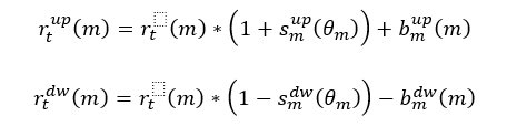
Regarding [C], EIOPA has confirmed its previous advice dated 2018 (relative shift approach), highlighting the need of modifying the IR risk calibration

The 3-years gradual implementation period would be reviewed in light of the proposed changes on the Risk Free Rates reported in [A] and [B].

Regarding [D], EIOPA has proposed to introduce tools to address systemic risk in the insurance sector by adding a general article to the SII Directive, to achieve consistency and coherence with the micro-prudential approach. NSAs should have the power to set a capital surcharge to address sources of systemic risk, to define soft thresholds for action at market level if an exposure increases dramatically and to impose a temporary restriction on surrender rights for policyholders. NSAs can require systemic risk management plans and all firms should be required to draft liquidity risk management plans, unless they obtain a waiver. The ORSA principle will be changed to explicitly include macro-prudential concerns. EIOPA has also proposed to:

• require firms with a high market share to develop a recovery plan
• set an officially designated administrative resolution authority in each member state
• provide the NSAs with resolution powers of: prohibiting bonus payments to senior management; withdrawing the licence to write new business and put all or part of existing business into run-off; selling or transferring shares, assets and liabilities to third parties; restricting the rights of policyholders to surrender policies; suspending payments to unsecured creditors; until the point of taking control of the entity.