When[1] the euro was created 20 years ago it was hailed as one of the most important turning points in the history of the international monetary system…
https://www.ecb.europa.eu//press/key/date/2019/html/ecb.sp190917~9b63e0ea23.en.html
When[1] the euro was created 20 years ago it was hailed as one of the most important turning points in the history of the international monetary system…
https://www.ecb.europa.eu//press/key/date/2019/html/ecb.sp190917~9b63e0ea23.en.html

Le attività di raccolta dei depositi e di impiego (credito) ai clienti sono cruciali per tutte le banche commerciali. In primis, perché le banche sono le uniche istituzioni finanziarie che possono avere un deposito, ad esempio nella forma del conto corrente. In secondo luogo, perché l’attività del credito permetterà di trasformare il deposito, che può essere ritirato in ogni momento e quindi ha una scadenza di breve termine, in un investimento con una scadenza temporale di lungo termine (es. mutuo). Da questo mismatch temporale proviene la maggiore fonte di guadagno delle banche, fintanto che la curva dei tassi di interesse prevede che venga remunerato un investimento a lungo termine più di uno a breve termine per corrispondere un premio al tempo e all’incertezza dell’investimento. Dal punto di vista della banca tale mismatch temporale è fonte di guadagno ma anche fonte di rischi, in particolare il rischio di liquidità e il rischio di tasso di interesse. Il primo riguarda l’incertezza relativa a quando e quanto verranno ritirati i depositi, o quando e quanto verranno ripagati prima del tempo previsto contrattualmente il debito verso la banca (e.g. prepagamento di mutui), facendo affluire/defluire con maggiore velocità la liquidità della banca. Il secondo tipo di rischio riguarda l’incertezza sul tasso con cui verranno remunerati i depositi ed il tasso di impiego dei crediti; entrambi i tassi dipendono dalla curva dei rendimenti e dai movimenti al rialzo/ribasso che potranno avvenire in futuri. Entrambi i rischi possono essere mitigati se la banca comprende il comportamento dei clienti e, tramite un modello, può prevedere quale sia l’ammontare di depositi stabili ed insensibili nel tempo o prevedere quale sia l’ammontare di prepagamenti. In conclusione, la redditività ed il rischio di liquidità e di tasso di interesse sono profondamente influenzati dal comportamento dei clienti e dai modelli interni utilizzati per gestire prospetticamente i rischi e la redditività futura.
Recentemente con Umberto Crespi abbiamo scritto un libro[1] dedicato ai modelli comportamentali, alla natura e corretta impostazione delle assunzioni usate nei modelli che hanno il fine di gestire il disallineamento (mismatch) tra i depositi/impieghi ed il relativo rischio di liquidità e tasso di interesse. Sono modelli statistici e matematici che si dividono, per semplicità, in due macro-categorie: i modelli per i depositi e quelli per il prepagamento. I primi mirano a stimare quale sia la parte di depositi che possa essere considerata come una fonte stabile di finanziamento e quale parte dei volumi sono insensibili alle variazioni dei tassi di interesse. I secondi, invece, sono modelli che stimano la probabilità ed il volume di finanziamenti (e.g. mutui) che sarà prepagato dal cliente. Il prepagamento può essere parziale o totale e, in entrambi i casi, modifica le rate contrattualmente previste. Quest’ultimo comportamento ha effetti importanti per l’intero portafoglio di crediti della banca malgrado sia stimato a livello di singolo evento (un mutuo). In particolare i modelli di prepagamento sono diventati rilevanti in paesi, come l’Italia, che hanno abolito la normativa vincolante il rapporto contrattuale univoco con la banca dando la possibilità di estinguere, prepagare o surrogare senza costi aggiuntivi (Decreto Bersani l. legge 2 aprile 2007, n. 40).
L’output dei modelli è rilevante per misurare e gestire il rischio di tasso di interesse ma anche per comprendere la redditività delle banche. In particolare, il modello dei depositi stima quale sia l’ammontare di prelievi che verranno effettuati dai conti correnti o, viceversa, qual è l’ammontare di depositi che non verrà prelevato, in un arco temporale di un anno o anche di più. Allo stesso tempo considera una probabilità di tali uscite e, per essere conservativi, di solito si prende il 95% o il 99% dei possibili scenari futuri. Facciamo un esempio: se sul conto corrente un cliente ha 1.000 euro, il modello dovrà prevedere quale sia l’ammontare, o la percentuale dei 1.000 euro, che sarà ancora sul conto corrente tra un anno o due anni o anche dieci anni. E tale percentuale deve essere prudente, nel senso che il modello deve considerare periodi di stress in cui, per diversi motivi, il conto corrente non è più alimentato da uno stipendio o una pensione ma ci sono sole uscite. Mettiamo che il risultato del modello con un orizzonte temporale di dieci anni e un livello di confidenza del 95% sia 300 euro. Di conseguenza la banca potrà investire, ad esempio in un mutuo, 300 euro prestandoli ad un cliente con un orizzonte di dieci anni, ed essere certa al 95% che non dovrà reperire altrove, ovvero sui mercati finanziari, 300 euro qualora il cliente richieda il proprio deposito indietro. Il secondo obiettivo del modello dei depositi è stimare, sempre con un certo livello di confidenza, quale parte di questi 300 euro depositati è insensibile al variare dei tassi di interesse. Assumiamo che il deposito sia remunerato con un tasso di interesse pari allo 0.1% e che il modello preveda per quel cliente un volume insensibile ai tassi di interesse pari a 200 euro. Questo significa che se i tassi di interesse nei prossimi dieci anni aumenteranno o diminuiranno solo 100 euro dovranno cambiare remunerazione a causa della fluttuazione mentre 200 euro riceveranno sempre lo 0.1%. Chiaramente, questo esempio non vale per un singolo correntista e bisogna osservare il fenomeno a livello di portafoglio, ovvero osservando tutti i clienti nel loro insieme o in sotto-insiemi effettuando l’analisi per il cluster Retail, Private o nel mondo delle imprese segregando le piccole dalle medie/grandi imprese.
Chiarito questo obiettivo, è importante capire le cause, ovvero le variabili esplicative del modello, che possono spiegare come mai il cliente con 1.000 euro sul conto utilizzerà con il 95% di probabilità nei prossimi dieci anni il 70% di quest’ultimi e chiederà, per l’80% di questo deposito, di rivedere al rialzo le condizioni contrattuali se i tassi di interesse di mercato aumenteranno, o viceversa, si vedrà la richiesta da parte della banca di diminuire la remunerazione dei depositi se i tassi scenderanno.
Usando l’econometria, congiuntamente alla logica economica, si crea il mix perfetto che consente al modello di assumere che gli eventi storici osservati siano predittivi del futuro in termini sia di dimensioni sia di impatto per le banche. Per questo motivo è importante avere un database utile alla stima del modello con una profondità storica di almeno 3-5 anni, una granularità dei dati che storicizzi il depositi medio mensile (quello giornaliero è troppo di dettaglio per l’obiettivo del modello), una capacità di aggregare i clienti in funzione dell’appartenenza al settore Retail, Private, small-business, grandi imprese o banche, e che includa per ognuno di essi la remunerazione dei depositi.
Seguendo la teoria economica, ognuno di noi detiene depositi sul conto corrente in funzione delle transazioni attese (componente transazionale) quali le spese per affitto, ristoranti o vestiti, per gestire le future transazioni (componente risparmio) o per investire (componente speculativa). Per questo motivo il modello dovrà considerare quelle variabili che possono spiegare la componente transazionali, di risparmio o speculativa. Tali variabili sono microeconomiche ed aiutano a spiegare la componente transazionale e di risparmio, quali il salario e la ricchezza finanziaria del cliente, il costo opportunità di muovere il deposito verso altre forme di investimento, il livello di competizione tra le banche o la presenza/assenza di una trattenuta per muovere la liquidità tra un conto corrente e un altro. In secondo luogo, le variabili macroeconomiche come l’andamento del PIL, dell’inflazione, dei salari e della disoccupazione sono utili a capire le componenti transazionali e di risparmio mentre l’andamento dei mercati finanziari (tassi di interesse, azionariato e obbligazionario) sono fondamentali per capire la componente speculativa. Non da ultimo, ci sono altre variabili che possono essere utili a prevedere quanti volumi saranno stabili ed insensibili ai tassi, e dipendono dalla banca ovvero la presenza di una strategia di business o di marketing che può incentivare/disincentivare l’utilizzo del deposito per fini transazionali o speculativi e rendendo più o meno appetibile il deposito su conto corrente.
Una volta comprese che tutte queste variabili possono essere rilevanti, diventa fondamentale l’analisi economica di quali, tra queste, siano più utili a predire il comportamento del cliente. Per questo motivo, nel libro suggeriamo di scegliere un modello semplice rispetto ad uno più complesso in funzione della qualità del database, ovvero della capacità di incrociare i dati con le variabili predittive. Un modello semplice utilizzerà, ad esempio, la serie storica dei volumi del conto corrente e ne prenderà un minimo o analizzerà qual è stata la variabilità minima-massima negli ultimi dieci anni assumendo che la stessa si potrà ripresentare nei prossimi dieci anni. Al contrario, un modello più complesso andrà ad integrare i depositi sul conto corrente dei clienti con il valore della ricchezza finanziaria e l’ammontare di investimenti (portafoglio titoli) cercando una relazione tra l’allocazione della ricchezza finanziaria tra il conto corrente ed il portafoglio titoli con l’andamento delle variabili finanziarie o del costo opportunità con altri prodotti di investimento.
Una volta ottenuto l’output, da un modello semplice o da uno più complesso, molti attori all’interno dei vari dipartimenti della banca ne faranno uso. E per questo motivo i modelli comportamentali sono importanti all’interno di tutto il processo bancario.
In primis, il dipartimento di tesoreria della banca, il quale utilizzerà l’ammontare di volumi stabili per la gestione del rischio di liquidità, il dipartimento di finanza e/o risk management per sapere quanta parte dei depositi potranno essere investiti in mutui a tasso fisso così da immunizzare la banca dal rischio tasso di interesse, o per stabilire il prezzo interno di trasferimento dei fondi ovvero la remunerazione dei depositi e dei mutui tra la tesoreria e le unità di business. Infine, il dipartimento di pianificazione per prospettare la redditività complessiva all’interno del piano industriale o il dipartimento che cura la relazioni con gli investitori i quali sono interessati a capire quale sia la redditività della banca. Per ultimo, questi modelli sono oggetto di attenzione da parte della vigilanza bancaria, ECB, e degli audit interni che, insieme al dipartimento di validazione dei modelli interni, si occuperà di verificare la corretta implementazione e stima dei modelli.
[1] A Guide to Behavioural Modelling – Risk.Net

L’iniziativa di Finriskalert.it “Il termometro dei mercati finanziari” vuole presentare un indicatore settimanale sul grado di turbolenza/tensione dei mercati finanziari, con particolare attenzione all’Italia.
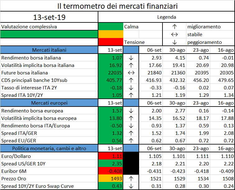
Significato degli indicatori
I colori sono assegnati in un’ottica VaR: se il valore riportato è superiore (inferiore) al quantile al 15%, il colore utilizzato è l’arancione. Se il valore riportato è superiore (inferiore) al quantile al 5% il colore utilizzato è il rosso. La banda (verso l’alto o verso il basso) viene selezionata, a seconda dell’indicatore, nella direzione dell’instabilità del mercato. I quantili vengono ricostruiti prendendo la serie storica di un anno di osservazioni: ad esempio, un valore in una casella rossa significa che appartiene al 5% dei valori meno positivi riscontrati nell’ultimo anno. Per le prime tre voci della sezione “Politica Monetaria”, le bande per definire il colore sono simmetriche (valori in positivo e in negativo). I dati riportati provengono dal database Thomson Reuters. Infine, la tendenza mostra la dinamica in atto e viene rappresentata dalle frecce: ↑,↓, ↔ indicano rispettivamente miglioramento, peggioramento, stabilità rispetto alla rilevazione precedente.
Disclaimer: Le informazioni contenute in questa pagina sono esclusivamente a scopo informativo e per uso personale. Le informazioni possono essere modificate da finriskalert.it in qualsiasi momento e senza preavviso. Finriskalert.it non può fornire alcuna garanzia in merito all’affidabilità, completezza, esattezza ed attualità dei dati riportati e, pertanto, non assume alcuna responsabilità per qualsiasi danno legato all’uso, proprio o improprio delle informazioni contenute in questa pagina. I contenuti presenti in questa pagina non devono in alcun modo essere intesi come consigli finanziari, economici, giuridici, fiscali o di altra natura e nessuna decisione d’investimento o qualsiasi altra decisione deve essere presa unicamente sulla base di questi dati.

Last April the European Council and Parliament approved one amendment to the calculation of the Volatility Adjustment (VA): the trigger for the Country VA has been moved from 100 to 85bps. This change is now being reviewed and will be published on the Official Journal of the European Union after the summer break. Once published, the Member States will have 6 months to include it in the local regulation.
The VA is one of the LTG (Long Term Guarantee) measures under SII which aims to ensure the appropriate treatment of insurance products with long term guarantees by dampening irrational market movements that would result in unjustified credit spreads. Unfortunately, according to the Italian insurance Companies and the Italian Regulator (IVASS), its mechanism has never been as effective as hoped. The Companies feared that the change they have been requesting for long would have only been set in place in 2020, together with the revision of the SII framework but, luckily, it has been recently approved during the vote of the ESA’s review.
The SII directive requires that both Assets and Liabilities are valued at a “fair price” and these quantities are then used to calculate both the OF (Own Funds) and the SCR (Solvency Capital Requirement) of a given firm. The business model of Insurance Companies is usually long termed, being their liabilities characterized by quite high durations. To be matched and with the aim of getting proper yields, Insurance Companies tend to invest in long term assets that, in this framework, suffer an “artificial level of volatility” of the spreads, which is short termed. The “artificial volatility” comes from non-default related changes in market values of bonds, like for instance the liquidity changes. However, since Insurance Companies have long-term guarantees and aim to hold their assets accordingly, it is rational to think that their OF and SCR should not be affected by those temporary changes. The VA is meant to offset this improper effect: when the spreads rise (and the value of the Assets falls down), the VA, applied on top of the Risk Free yield curve, increases as well (reducing the value of the Liabilities).
The VA is published on a monthly base by EIOPA and is made up of two components:
both are reduced by an application ratio of 65% and then summed up.
The Currency VA is based on the 65% of the risk-corrected spreads between the interest rate that could be earned from a reference portfolio of assets and the risk free interest rates without any adjustment. A Currency-specific reference portfolio is used to determine the portfolio yield spread over the relevant risk free rate less the portion related to default or credit risk; the result of the calculation is referred to as the risk corrected currency spread. The portion related to default or credit risk is referred to as the “risk correction” (or fundamental spread) and is based on a percentage of the Long Term Average Spreads (LTAS) observed in the past 30 years (it describes the portion of the spread that is attributable to a realistic assessment of expected losses, unexpected credit risk or any other risk). The VA could turn negative when observed spreads are lower than the historical spreads, however is limited to the level of the risk correction: in practice it is expected that bonds maintain a positive spread as investors can hold swaps as an alternative (which reduce credit risk).
In addition to the Currency VA, a Country VA can be applied under specific circumstances. The Country VA is aimed at capturing situations where a country suffers a credit downgrade, which would lead to significant drop in government bonds from that country. The Country VA only applies when the risk corrected country spread is greater than twice the risk-corrected currency spread and the risk correct country spread is greater than 85 (previously 100) bps.
The following chart shows a case study carried out by ANIA (the Italian National Association of Insurance Firms): the blue dots depict the currency VA value in the recent history and the red dots the corresponding total VA value when the country part is triggered; the red values in the filled squares show the times in history when the country VA would have been triggered if a threshold of 85 had been used in place of the former 100bps. It is clear that a lower threshold would have allowed for a more ongoing and coherent effect:
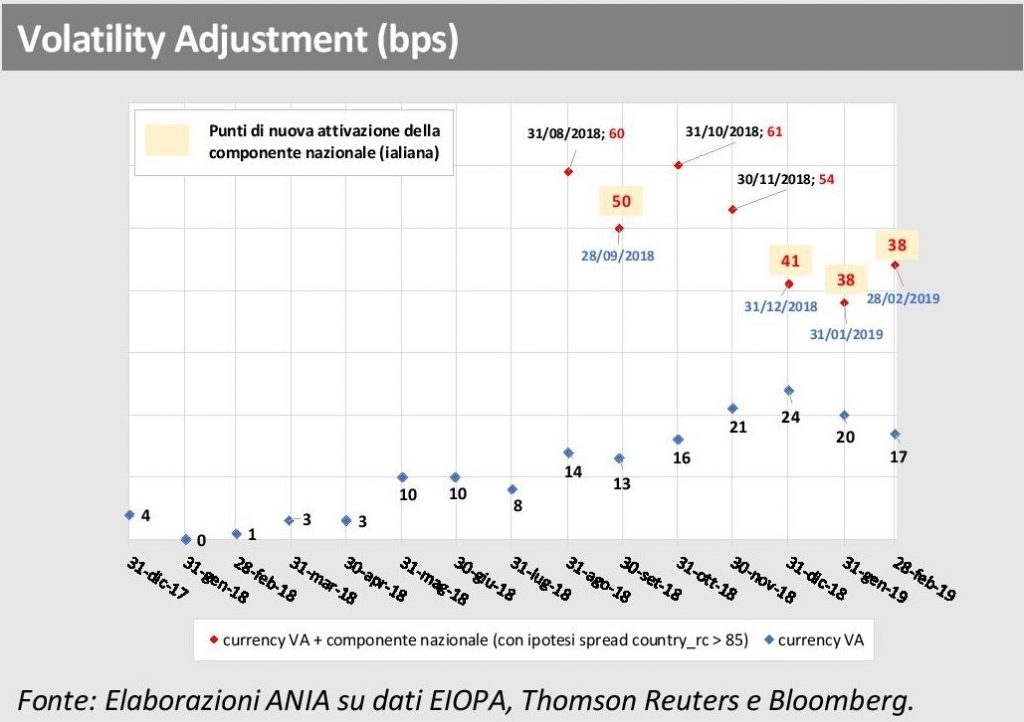
However, ANIA stated that this achievement is a short term solution and that the mechanism of the VA must be reviewed from the basis.
Lastly, as already recalled, the VA is calculated based on a pre-defined reference investment portfolio, representing an average European insurer. While the use of a generic representative asset portfolio and the resulting adjustment on the liability discounting curve are desirable ensuring convergence in the calculation of the Solvency II ratio, it may not really be appropriate for firms that show different durations or assets allocations.
Spanish banking giant Santander says it has become the first institution to use a public blockchain to manage all aspects of a bond issue…
The French finance minister has said the nation plans to block Facebook’s Libra cryptocurrency in the EU over concerns that it poses a threat to the sovereignty of national currencies…
https://www.coindesk.com/france-says-it-will-block-facebook-libra-in-europe-report
The Governing Council of the European Central Bank (ECB) today decided to introduce a two-tier system for reserve remuneration…
https://www.ecb.europa.eu//press/pr/date/2019/html/ecb.pr190912_2~a0b47cd62a.en.html
The European Union’s (EU) banking, insurance, pensions and securities sectors continue to face a range of risks…

L’iniziativa di Finriskalert.it “Il termometro dei mercati finanziari” vuole presentare un indicatore settimanale sul grado di turbolenza/tensione dei mercati finanziari, con particolare attenzione all’Italia.
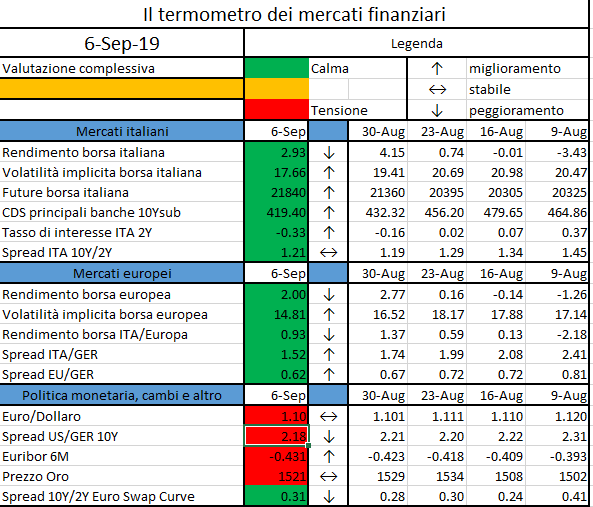
Significato degli indicatori
I colori sono assegnati in un’ottica VaR: se il valore riportato è superiore (inferiore) al quantile al 15%, il colore utilizzato è l’arancione. Se il valore riportato è superiore (inferiore) al quantile al 5% il colore utilizzato è il rosso. La banda (verso l’alto o verso il basso) viene selezionata, a seconda dell’indicatore, nella direzione dell’instabilità del mercato. I quantili vengono ricostruiti prendendo la serie storica di un anno di osservazioni: ad esempio, un valore in una casella rossa significa che appartiene al 5% dei valori meno positivi riscontrati nell’ultimo anno. Per le prime tre voci della sezione “Politica Monetaria”, le bande per definire il colore sono simmetriche (valori in positivo e in negativo). I dati riportati provengono dal database Thomson Reuters. Infine, la tendenza mostra la dinamica in atto e viene rappresentata dalle frecce: ↑,↓, ↔ indicano rispettivamente miglioramento, peggioramento, stabilità rispetto alla rilevazione precedente.
Disclaimer: Le informazioni contenute in questa pagina sono esclusivamente a scopo informativo e per uso personale. Le informazioni possono essere modificate da finriskalert.it in qualsiasi momento e senza preavviso. Finriskalert.it non può fornire alcuna garanzia in merito all’affidabilità, completezza, esattezza ed attualità dei dati riportati e, pertanto, non assume alcuna responsabilità per qualsiasi danno legato all’uso, proprio o improprio delle informazioni contenute in questa pagina. I contenuti presenti in questa pagina non devono in alcun modo essere intesi come consigli finanziari, economici, giuridici, fiscali o di altra natura e nessuna decisione d’investimento o qualsiasi altra decisione deve essere presa unicamente sulla base di questi dati.

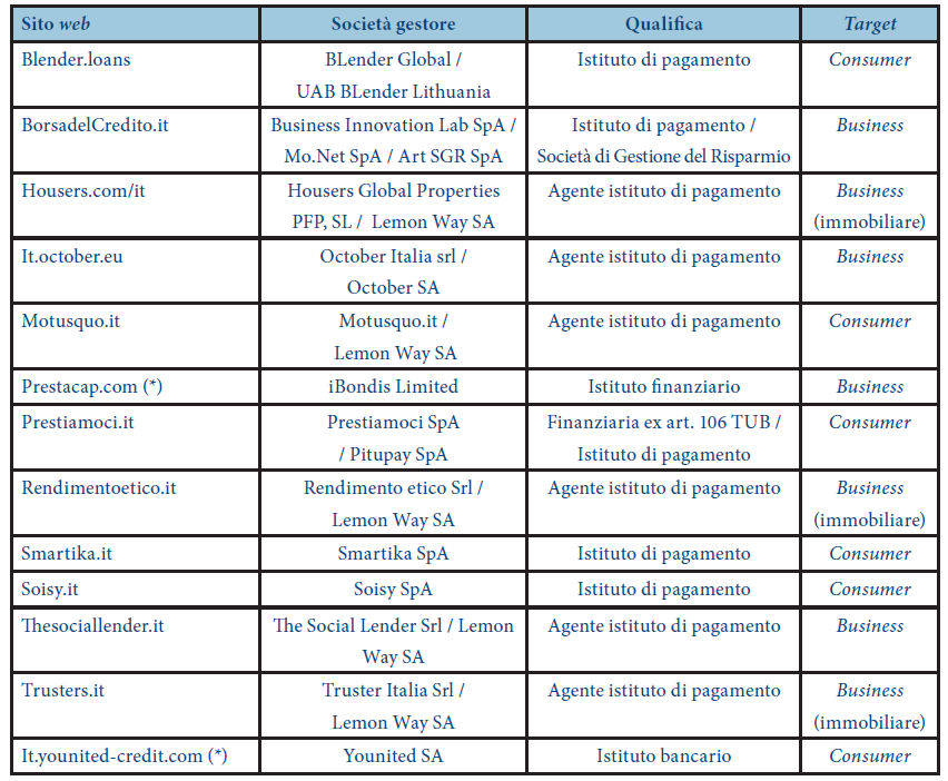
Il 4° Report italiano sul CrowdInvesting realizzato dalla School of Management del Politecnico di Milano permette di delineare lo stato attuale dell’arte in Italia riguardante il fenomeno del lending crowdfunding, ovvero l’opportunità di ottenere un prestito attraverso una piattaforma Internet (finanziata dalla ‘folla’ diffusa ma anche da investitori istituzionali).
Aggiornato al 30 giugno 2019, il report documenta la presenza di 13 portali di lending crowdfunding (si veda la Tabella 1), di cui 6 destinati al finanziamento di persone fisiche (consumer) e 7 rivolti al finanziamento di imprese (business). A tal proposito, è interessante notare che in ambito business ben 3 piattaforme su 7 sono specializzate nel segmento real estate. Inoltre, tre piattaforme business in data 30 giugno erano sulla rampa di lancio pronte a partire.
In riferimento al modello di investimento adottato, aumenta nel business lending il numero di piattaforme che adottano il modello ‘diretto’ (cioè dando possibilità di scelta immediata al finanziatore su come allocare i prestiti) mentre si consolida l’utilizzo del modello ‘diffuso’ (cioè con la suddivisione del denaro investito su tanti crediti diversificati) in ambito consumer.
A tal fine vale la pena sottolineare che i prestiti erogati dalle piattaforme sono generalmente privi di garanzie. A tal proposito un elemento di differenziazione tra i portali è dato dalla presenza o meno di fondi di protezione, istituiti per far fronte a eventuali inadempienze dei soggetti finanziati. Tali fondi, insieme alla garanzia pubblica del Fondo statale per le PMI, agiscono da tutela per i prestatori, incentivando questi ultimi a effettuare più investimenti. Il fondo in questione viene creato depositando una fee addizionale che viene richiesta solitamente ai finanziati (agli investitori nel caso di BLender, MotusQuo e Soisy), rendendo pertanto più oneroso l’accesso al capitale per i richiedenti.
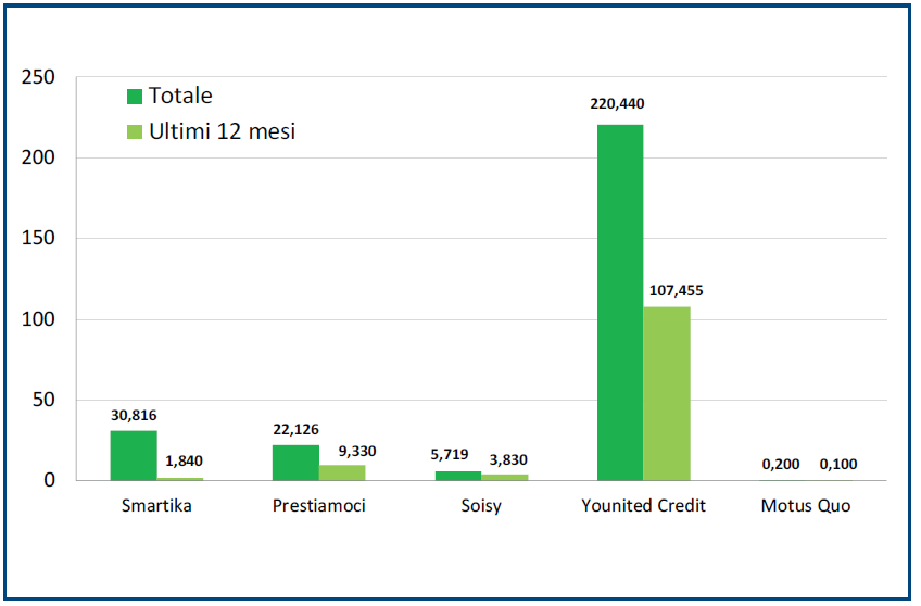
In Italia, i volumi cumulati raccolti tramite lending crowdfunding ammontano in totale a € 435 milioni, in particolare € 279 milioni per il segmento consumer (di cui € 122,5 milioni nell’ultimo anno) e € 156 milioni per la parte business (di cui € 84 milioni nell’ultimo anno). È rilevante osservare che entrambi i segmenti sono in crescita, con flussi rispettivamente in aumento del 40% (consumer) e 48% (business) rispetto all’anno precedente.
In ambito consumer, come la Figura 1 evidenzia, la piattaforma leader si conferma Younited Credit (che però non raccoglie dalla ‘folla’ di Internet), la quale ha complessivamente erogato prestiti per un valore superiore a € 220 milioni, di cui € 107 milioni solo negli ultimi 12 mesi. Tuttavia, se spostiamo l’attenzione sul numero di prestatori attivi, Smartika detiene il primato con ben 6541 finanziatori attivi.
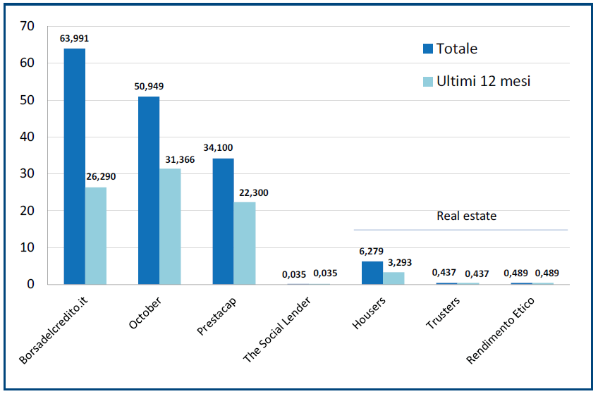
Per quanto invece concerne il business lending, la Figura 2 mostra che tre sono i principali potali in termini di valore del raccolto: Borsadelcredito.it, October e Prestacap. In particolare, il primo posto è occupato da Borsadelcredito.it con € 64,0 milioni mentre October si posiziona al secondo posto ma è il portale che ha raccolto di più negli ultimi 12 mesi.
Con lo sguardo rivolto al futuro, se da un lato è auspicabile aspettarsi che il business lending possa eguagliare i volumi del segmento consumer, dall’altro lato rimane più complesso, ma allo stesso tempo urgente, l’intervento sul quadro normativo del lending crowdfunding. Difatti, numerose questioni, tra cui la recente opportunità per i portali di equity crowdfunding di collocare debito, pongono l’intervento normativo come una delle priorità finalizzate a un’ulteriore crescita del fenomeno in linea con gli altri Paesi europei.
