Our part is to support early-stage projects that are helping to create the building blocks and infrastructure for larger utility and enabling growth in the blockchain market…
Apr
13
2019
Our part is to support early-stage projects that are helping to create the building blocks and infrastructure for larger utility and enabling growth in the blockchain market…
The euro area economy expanded at a slower pace in 2018, following robust growth in the previous year…
https://www.ecb.europa.eu//press/key/date/2019/html/ecb.sp190412~8acda1aa03.en.html
This course aims at providing an introductory and broad overview of the field of Machine Learning (ML) with the focus on applications on Finance.
Detailed Program:
1.Introduction to Financial problems and their classical solutions
2.Introduction to Machine Learning
– Supervised Learning
– Overview of regression and classification techniques
– Financial applications: price prediction, modeling bank failures
– Unsupervised Learning
– Overview of clustering and dimensionality reduction techniques
– Financial applications: stock returns, estimation of equity correlation matrix
– Reinforcement Learning
– Overview of value-based and policy-based techniques
– Financial applications: option pricing, stock trading
Venue: Department of Mathematics, Politecnico di Milano
Time Table:
Introduction to Financial applications (Baviera, Marazzina, Rroji):
June 13: 9:30-12:00, 14:30-17:00 (Prof. Marazzina)
June 17: 9:30-12:00 (Prof. Baviera), 14:30-17:00 (Prof. Rroji)
June 18: 9:30-12:00 (Prof. Baviera), 14:30-17:00 (Prof. Rroji)
Machine Learning (Restelli, Baviera):
June 20, 21, 25, 27, 28: 10:00-13:00 (Prof. Restelli)
July 1: 15:00-17:00 (Prof. Baviera)
For information: daniele.marazzina@polimi.it

L’iniziativa di Finriskalert.it “Il termometro dei mercati finanziari” vuole presentare un indicatore settimanale sul grado di turbolenza/tensione dei mercati finanziari, con particolare attenzione all’Italia.
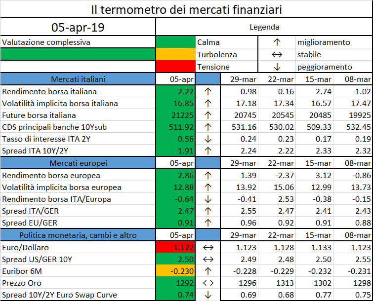
Significato degli indicatori
I colori sono assegnati in un’ottica VaR: se il valore riportato è superiore (inferiore) al quantile al 15%, il colore utilizzato è l’arancione. Se il valore riportato è superiore (inferiore) al quantile al 5% il colore utilizzato è il rosso. La banda (verso l’alto o verso il basso) viene selezionata, a seconda dell’indicatore, nella direzione dell’instabilità del mercato. I quantili vengono ricostruiti prendendo la serie storica di un anno di osservazioni: ad esempio, un valore in una casella rossa significa che appartiene al 5% dei valori meno positivi riscontrati nell’ultimo anno. Per le prime tre voci della sezione “Politica Monetaria”, le bande per definire il colore sono simmetriche (valori in positivo e in negativo). I dati riportati provengono dal database Thomson Reuters. Infine, la tendenza mostra la dinamica in atto e viene rappresentata dalle frecce: ↑,↓, ↔ indicano rispettivamente miglioramento, peggioramento, stabilità rispetto alla rilevazione precedente.
Disclaimer: Le informazioni contenute in questa pagina sono esclusivamente a scopo informativo e per uso personale. Le informazioni possono essere modificate da finriskalert.it in qualsiasi momento e senza preavviso. Finriskalert.it non può fornire alcuna garanzia in merito all’affidabilità, completezza, esattezza ed attualità dei dati riportati e, pertanto, non assume alcuna responsabilità per qualsiasi danno legato all’uso, proprio o improprio delle informazioni contenute in questa pagina. I contenuti presenti in questa pagina non devono in alcun modo essere intesi come consigli finanziari, economici, giuridici, fiscali o di altra natura e nessuna decisione d’investimento o qualsiasi altra decisione deve essere presa unicamente sulla base di questi dati.
Per le imprese del Regno Unito e Irlanda del Nord (di seguito UK)1 che operano nel settore delle assicurazioni contro i danni, l’Italia è il primo Paese dell’EU27 per numero di assicurati (9,7 mln) e per riserve tecniche (3 €/mld) e il quarto Paese per premi raccolti (1,7 €/mld)2…
The European Securities and Markets Authority (ESMA) has today published the framework for its third EU-wide Central Counterparties (CCPs) stress test…
To increase competitiveness is the main driver for higher potential growth. Member states have to pursue politics and establish institutions that stimulate the dynamics of a competitive private sector…
https://www.ecb.europa.eu//press/key/date/2019/html/ecb.sp190406~f2af7b707b.en.html
SWIFT, IBM, Ripple and around 100 other firms and organizations have joined a new blockchain association to promote adoption of the technology across the EU…

On the 26th of March 2019 IVASS has issued a press release communicating an update on the data related to the dormant life assurance policies: 208,863 contracts, amounting to 3.9 billion euros, have been “awakened” by the Italian Regulator.
Dormant life assurance policies are those that have not been collected by the beneficiaries and lie dormant at insurance undertakings until they become time-barred. The rights arising from those policies are barred after 10 years from the event (death or maturity), when the corresponding benefits are paid to the Dormant Accounts Fund. Dormant policies can be either contingent on death, if beneficiaries do not cash in the benefits because they may not be aware of the policy itself, or saving policies not collected upon maturity for any reason.
The extensive phenomenon of potentially dormant policies arose from both the shortcomings embedded in the procedures carried out by the undertaking when checking the deaths of insureds and identifying its beneficiaries and from the widespread use of generic formulations to indicate the beneficiaries when underwriting the contract.
To contrast and reduce this phenomenon, the Regulator has:
IVASS has started the investigation on dormant policies (first wave) back in 2017, publishing some important results on the 3rd September 2018. At that date, 187,493 policies amounting to 3.5 billion euros had already been “awakened” by matching the tax code of the insured people with the data stored in the tax-payers database by “Agenzia delle entrate” – Revenue Agency, the Italian IRS (Internal Revenue Service) – while other 900,000 contracts still had to be checked. The analysis, updated at the 31st of January 2019 and published on the 26th March 2019, shows that the Regulator has “awakened” other 21,370 policies, amounting to other 335 million euros. The table below, released by IVASS, reports the details of those policies and clarifies that, out of the original 900,000 contracts, 13,171 still must be verified. These ones are related to old policies, with no obligation of indicating the tax code of the insured and with no clear indication of the beneficiary. IVASS suggests in those cases to use specialized companies to retrieve the missing information. The rest of the policies (873,000 = 96%* 900,000) have correctly not been paid being the insured person alive at maturity or the policy insolvent (i.e. the policyholder has stopped the payment of the premiums, causing the resolution of the contract)
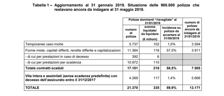
In addition to the 21,370 “awakened” policies, there are other 436 contracts, amounting to 7 million euros, that have become time-barred and should be paid to the Dormant Account Fund.
IVASS is now waiting for a feedback on other policies investigated in the last months (second wave), whose data were provided by the undertaking on the 30th October 2018. Indeed, on the 3rd September 2018, the regulator decided to extend the perimeter of the analysis to contracts expired in the period 2001-2006 and to those expired in 2017 and not yet settled. By the end of May 2019 the undertakings will have to give IVASS a feedback on the cases highlighted by the regulator, with a dead insured the undertakings were not aware of.
IVASS is now investigating the policies (third wave) whose data were provided by EEA foreign undertakings last 28th February 2019. These policies are related to contracts either expired between 2001 and 2017 or to whole life policies outstanding at 31 December 2018. The aim of this analysis is to offer the same level of protection to all the beneficiaries, independently of the nationality of the undertaking.
Following a proposal from IVASS, a new law has been issued on December 2018: every insurance company operating in Italy shall check at the end of each solar year whether its insured are still alive. If not, the undertaking shall pay the beneficiary and inform the Regulator by the next 31st March. The first check will be carried out next 31st December 2019.
L’iniziativa di Finriskalert.it “Il termometro dei mercati finanziari” vuole presentare un indicatore settimanale sul grado di turbolenza/tensione dei mercati finanziari, con particolare attenzione all’Italia.
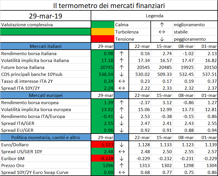
Significato degli indicatori
I colori sono assegnati in un’ottica VaR: se il valore riportato è superiore (inferiore) al quantile al 15%, il colore utilizzato è l’arancione. Se il valore riportato è superiore (inferiore) al quantile al 5% il colore utilizzato è il rosso. La banda (verso l’alto o verso il basso) viene selezionata, a seconda dell’indicatore, nella direzione dell’instabilità del mercato. I quantili vengono ricostruiti prendendo la serie storica di un anno di osservazioni: ad esempio, un valore in una casella rossa significa che appartiene al 5% dei valori meno positivi riscontrati nell’ultimo anno. Per le prime tre voci della sezione “Politica Monetaria”, le bande per definire il colore sono simmetriche (valori in positivo e in negativo). I dati riportati provengono dal database Thomson Reuters. Infine, la tendenza mostra la dinamica in atto e viene rappresentata dalle frecce: ↑,↓, ↔ indicano rispettivamente miglioramento, peggioramento, stabilità rispetto alla rilevazione precedente.
Disclaimer: Le informazioni contenute in questa pagina sono esclusivamente a scopo informativo e per uso personale. Le informazioni possono essere modificate da finriskalert.it in qualsiasi momento e senza preavviso. Finriskalert.it non può fornire alcuna garanzia in merito all’affidabilità, completezza, esattezza ed attualità dei dati riportati e, pertanto, non assume alcuna responsabilità per qualsiasi danno legato all’uso, proprio o improprio delle informazioni contenute in questa pagina. I contenuti presenti in questa pagina non devono in alcun modo essere intesi come consigli finanziari, economici, giuridici, fiscali o di altra natura e nessuna decisione d’investimento o qualsiasi altra decisione deve essere presa unicamente sulla base di questi dati.
