EIOPA has recently published the risk dashboard (RDB) update at January 2019.
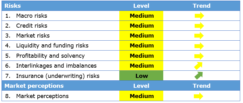
The RDB is published on a quarterly basis, showing the level of risk for 8 (=7+1) risk categories. The latest outcome is:
Some comments
1.Macro risks [medium, stable]
This is an overarching category affecting the whole economy, which considers economic growth, monetary policies, consumer price indices and fiscal balances.
The economic environment remains fragile because of the negative forecast on the GDP growth, which has been revised downwards across major economic areas (Euro Area, Switzerland, US and BRICS) and the potential reduction of the accommodative stance of monetary policy. On the other hand, the swap rates keep on being low and the indicator on 10y swap rates even decreases from the previous quarter (1.30%, -0.13%), due to slight declines in swap rates for all the currencies considered (EUR, GBP, CHF, USD). The unemployment rate remains quite stable from the previous quarter (6.0%, -0.1%), meaning that the labour market recovery is potentially starting to slow down. The inflation (CPI) remains broadly unchanged from the previous quarter (1.92%, -0.06%).
2.Credit risks [medium, stable]
This category measures the vulnerability to the credit risk by looking at the relevant credit asset classes exposures combined with the associated metrics (e.g. government securities and credit spread on sovereigns). Compared to the previous assessment, the exposures of the Insurers in different asset classes remain quite stable and around
- 30% in European sovereign bonds, whose CDS spreads has slightly decreased
- 12.5% in non-financial corporate bonds, whose spreads have increased
- 8% in unsecured financial corporate bonds, whose spreads has considerably increased
- 3% in secured financial corporate bonds, whose spreads has substantially increased, even turning positive for the first time since 2017Q1
- 0.7% in loans and mortgages
3.Market risks [medium, stable]
This vulnerability of the insurance sector to adverse developments is evaluated based on the investment exposures, while the current level of riskiness is evaluated based on the volatility of the yields together with the difference between the investment returns and the guaranteed interest rates. The market risks remain stable, reflecting the stability of the portfolios’ allocations of insurers, where the volatility of the bonds, largest asset class (60% of exposure) and property (2.5% exposure), remain stable, while the volatility of the equity markets (7%) continues to increase.
4.Liquidity and funding risk [medium, stable]
The vulnerability to liquidity shocked is monitored measuring the lapse rate, the holding in cash and the issuance of catastrophe bonds (low volumes or high spreads correspond to a reduction in the demand which could forma a risk). The liquid assets ratio has registered a small decrease since the previous quarter, while issued bond volumes and the average ratio of coupons to maturity also reduced. Lapse rates in life business remained overall unchanged across the whole distribution since 2016; median lapse rates are still around 3%.
5.Profitability and solvency [medium, stable]
The solvency level is measured via SCR and quality of OF, while the profitability via return on investments / combined ratio for the life / non-life sectors. The SCR ratios for non-life solo companies have recorded a modest improvement since the last quarter (median value 209%, +2.5%). he median SCR ratio for life companies has decreased (183%, -4%), whereas the overall distribution has shifted upwards.
6.Interlinkages and imbalances [medium, increasing]
Interlinkages are assessed between primary insurers and reinsurers, insurance and banking sector and among the derivative holdings. The exposure towards domestic sovereign debt is considered as well. Interlinkages and imbalances risks has increased, but remaining at medium level in Q3 2018. Exposures to banks and other financial institutions has remained broadly stable, while exposures to insurers has increased due to corporate actions and M&A activity by some insurance groups.
7.Insurance (underwriting) risk [low, increasing]
Indicators for insurance risks are gross written premia, claims and losses due to natural catastrophes. The increase of the risk in this category is driven by increase in the premium growth of both life and non-life insurance together with an increase in the catastrophe loss ratio. For some line of business, some concerns are raised by both under pricing and under reserving, driven by competition.
8.Market perception [medium, stable]
The market perception remains constant at medium level. The quantities assessed are relative stock market performances (insurance stock outperformed the Stoxx 600: +1.5% life, +4% non-life), price to earnings ratio (decreased from the previous released: average from 13.1% to 11.6%), CDS spreads (median value increased from 61 to 68) and external rating outlooks (improved, with a portion of insurers with credit quality step =3 moving to 2).