La Banca d’Italia rivede al ribasso le stime sulla crescita del’economia italiana. Le proiezioni macro, elaborate da via Nazionale nell’ambito dell’esercizio coordinato dell’Eurosistema, mostrano una crescita del prodotto quest’anno del 2,6%, una frenata all’1,6% nel 2023 e una lieve accelerazione (all’1,8) nel 2024.
The European Securities and Markets Authority (ESMA), the EU securities markets regulator, today updates its risk assessment to account for the impacts on financial markets of Russia’s invasion of Ukraine and the deteriorating economic environment…
Russia’s war against Ukraine has severely hit confidence, caused energy and food prices to soar further and, together with pandemic-related disruptions in China, compounded existing supply chain pressures. These factors pose strong headwinds for the economic recovery in the euro area…
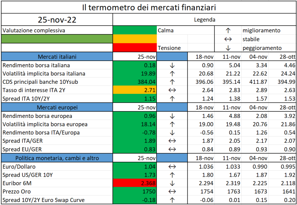
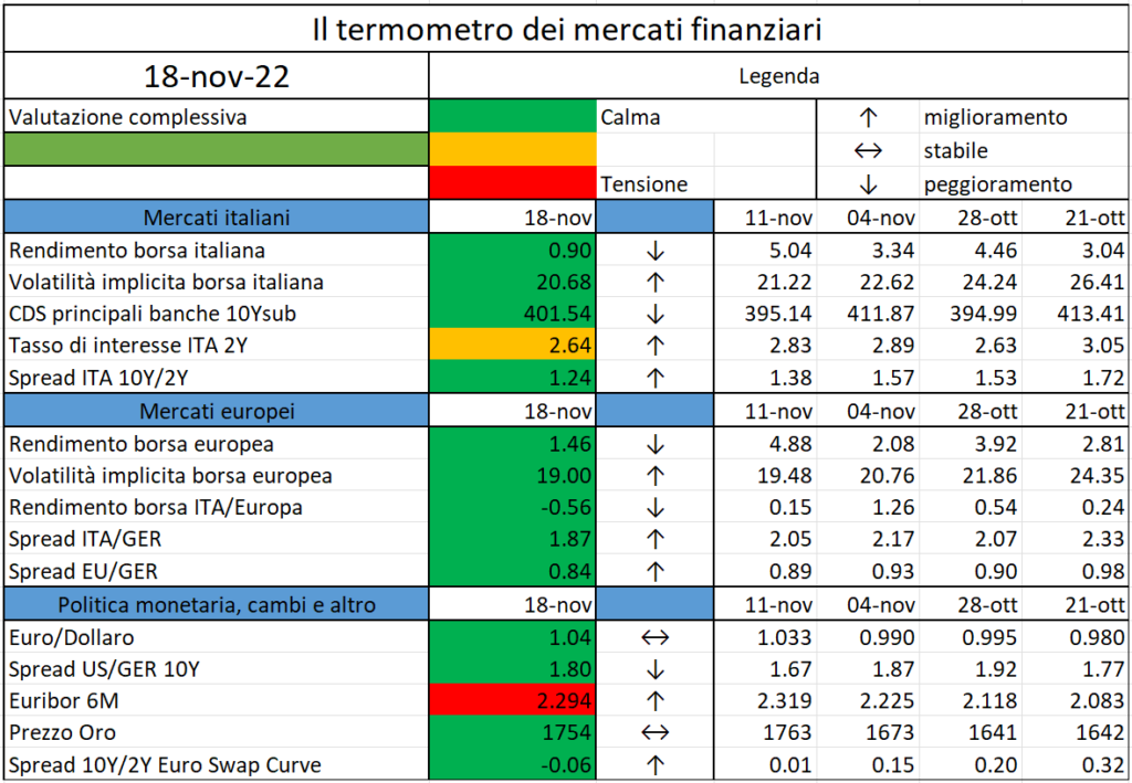
L’iniziativa di Finriskalert.it “Il termometro dei mercati finanziari” vuole presentare un indicatore settimanale sul grado di turbolenza/tensione dei mercati finanziari, con particolare attenzione all’Italia.
Significato degli indicatori
Rendimento borsa italiana: rendimento settimanale dell’indice della borsa italiana FTSEMIB;
Volatilità implicita borsa italiana: volatilità implicita calcolata considerando le opzioni at-the-money sul FTSEMIB a 3 mesi;
Future borsa italiana: valore del future sul FTSEMIB;
CDS principali banche 10Ysub: CDS medio delle obbligazioni subordinate a 10 anni delle principali banche italiane (Unicredit, Intesa San Paolo, MPS, Banco BPM);
Tasso di interesse ITA 2Y: tasso di interesse costruito sulla curva dei BTP con scadenza a due anni;
Spread ITA 10Y/2Y : differenza del tasso di interesse dei BTP a 10 anni e a 2 anni;
Rendimento borsa europea: rendimento settimanale dell’indice delle borse europee Eurostoxx;
Volatilità implicita borsa europea: volatilità implicita calcolata sulle opzioni at-the-money sull’indice Eurostoxx a scadenza 3 mesi;
Rendimento borsa ITA/Europa: differenza tra il rendimento settimanale della borsa italiana e quello delle borse europee, calcolato sugli indici FTSEMIB e Eurostoxx;
Spread ITA/GER: differenza tra i tassi di interesse italiani e tedeschi a 10 anni;
Spread EU/GER: differenza media tra i tassi di interesse dei principali paesi europei (Francia, Belgio, Spagna, Italia, Olanda) e quelli tedeschi a 10 anni;
Euro/dollaro: tasso di cambio euro/dollaro;
Spread US/GER 10Y: spread tra i tassi di interesse degli Stati Uniti e quelli tedeschi con scadenza 10 anni;
Prezzo Oro: quotazione dell’oro (in USD)
Spread 10Y/2Y Euro Swap Curve: differenza del tasso della curva EURO ZONE IRS 3M a 10Y e 2Y;
Euribor 6M: tasso euribor a 6 mesi.
I colori sono assegnati in un’ottica VaR: se il valore riportato è superiore (inferiore) al quantile al 15%, il colore utilizzato è l’arancione. Se il valore riportato è superiore (inferiore) al quantile al 5% il colore utilizzato è il rosso. La banda (verso l’alto o verso il basso) viene selezionata, a seconda dell’indicatore, nella direzione dell’instabilità del mercato. I quantili vengono ricostruiti prendendo la serie storica di un anno di osservazioni: ad esempio, un valore in una casella rossa significa che appartiene al 5% dei valori meno positivi riscontrati nell’ultimo anno. Per le prime tre voci della sezione “Politica Monetaria”, le bande per definire il colore sono simmetriche (valori in positivo e in negativo). I dati riportati provengono dal database Thomson Reuters. Infine, la tendenza mostra la dinamica in atto e viene rappresentata dalle frecce: ↑,↓, ↔ indicano rispettivamente miglioramento, peggioramento, stabilità rispetto alla rilevazione precedente.
Disclaimer: Le informazioni contenute in questa pagina sono esclusivamente a scopo informativo e per uso personale. Le informazioni possono essere modificate da finriskalert.it in qualsiasi momento e senza preavviso. Finriskalert.it non può fornire alcuna garanzia in merito all’affidabilità, completezza, esattezza ed attualità dei dati riportati e, pertanto, non assume alcuna responsabilità per qualsiasi danno legato all’uso, proprio o improprio delle informazioni contenute in questa pagina. I contenuti presenti in questa pagina non devono in alcun modo essere intesi come consigli finanziari, economici, giuridici, fiscali o di altra natura e nessuna decisione d’investimento o qualsiasi altra decisione deve essere presa unicamente sulla base di questi dati
Per conoscere il (probabile) futuro di una stock, l’AI studia i dati del passato. Antonio Simeone (Fondo Euklid): “Con le reti neurali ricaviamo informazioni qualitative. Chi le controlla dispone di un vantaggio competitivo”[Continua su HuffPost.it]
Following the overview provided in [3] “IFRS17 is coming soon”, this article focuses on a potential definition of Risk Adjustment (RA) that departs from the Risk Margin one under SII and provides a methodology for its release in the Income Statement (IS). The mathematical background is accompanied by numerical examples.
Under IFRS17 the total Liabilities are given by the sum of the Liability for Incurrent Claims (LIC), a reserve meant to cover the outstanding claims, and the Liability for Remaining Coverage (LRC). The latter is defined as the sum of the technical reserves, that, in turn, is given by the Present Value of Future Cash Flows (PVFCFs) plus the Risk Adjustment (RA), and the accountant reserve named Contract Service Margin (CSM). The RA is a provision for the risk, reflecting the level of compensation the insurer demands for bearing the uncertainty embedded in the amount and timing of CFs related to non-financial risks, excluding the operational one, as not directly generated by insurance contracts. The International Accounting Standard Board (IASB) has prescribed the need for the undertakings to disclose the confidence level chosen for the calculation, to show their degree of risk aversion, but has not specified a technique for the RA derivation, rather providing general characteristics it shall respect.
[B91] …the RA for non-financial risk shall have the following characteristics:
risks with low frequency and high severity will result in higher RA for non-financial risk than risks with high frequency and low severity
for similar risks, contracts with a longer duration will result in higher RA for non-financial risk than contracts with a shorter duration
risks with a wider probability distribution will result in higher Risk Adjustments for non-financial risk than risks with a narrower distribution
the less that is known about the current estimate and its trend, the higher will be the Risk Adjustment for non-financial risk
to the extent that emerging experience reduces uncertainty about the amount and timing of cash flows, RA for non-financial risk will decrease and vice versa.
The two most common techniques adopted to derive the RA are the Cost of Capital (CoC) approach and the Value at Risk (VaR) approach. As it appears to be quite complicated translating a confidence level into a CoC value (for the avoidance of doubt, the 6% CoC under SII is not equivalent to a quantile of 99.50%), many companies are opting for the second technique, deeply discussed in the following. The higher the RA, the higher the uncertainty around the projections. The article also describes the pros and cons of having a high or low value of Risk Adjustment and how its variation can be split into one part concerning the services already provided, and released to the IS, and another part concerning the future services and counted for in the CSM. Indeed, as shown by the following picture, this RA change, together with the Expected Claims, compares to the Actual Claims, to capture the non-economic variance.
To adopt a VaR approach, the undertaking shall define the perimeter of risks to analyse, the confidence level at which the VaR is measured, and its time horizon: indeed, the remaining lifetime of the contract must be considered when deriving a provision for the uncertainty of non-financial risks. A possible calculation of the RA can be run following these steps, from the bottom to the top:
the RA is defined as a n-years VaR, with n indicating the remaining lifetime of the pool of contract
the n-years VaR is derived from the 1-year VaR
the 1-year VaR is derived by aggregating 1-year univariate VaR (one for each risk considered)
this can be done, for example, by means of the SII LUR correlation matrix
each univariate 1-year VaR is defined as the change in PVFCFs (stressed – base) when a certain risk is stressed to a given confidence level, based on its distribution.
This methodology holds under the assumptions that
during the remaining n years of projection, the shocks of the underwriting risks are independent and identically distributed (i.i.d.), for instance with a Gaussian distribution
the distributions of the shocks and their confidence levels are transformed into distributions of stressed PVFCFs, as shown by this trivial example of direct linear dependency to the mortality risk
The outlined methodology is based on the following principles
the RA measures the uncertainty (variability) around the PVFPs value in the following n years
the uncertainty with a given confidence level a is measured as the VaR of PVFCFs returns (i.e., variations in its value) that are i.i.d. and distributed as Gaussians
the PVFCFs returns are directly linked to the shocks of the risks, that are distributed as Gaussians and whose value can be derived from the stress level defined by the SII directive (with an exception for the CAT risk, that can be kept at the SII level, for the sake of prudency)
This drives to the conclusion that
The idea behind the formula is that
the (multiperiodic) RA under IFRS17, similarly to the (one-period) RM under SII, is a provision for the uncertainty around the estimation of the underwriting risks, therefore a cushion to absorb unexpected changes in the PVFCFs driven by unexpected changes in the underwriting parameters
under SII the SCRRU measures the reduction of OF in a stressed combined scenarios with stresses pushed at a confidence level of 99.50% (1 every 200 years)
in each univariate dimension of underwriting risks (aggregated by the means of a correlation matrix), the Assets (A) stay the same and the univariate capital requirement corresponds to a change in Liabilities (L)
the Liabilities (L) establish a value (a price) for the insurance contract and the SCRRU provides a change in that price, so a return when compared to the base Liability value: for example, given Lbase=100 and Lstr=110, the SCRRU is defined as delta(L) = 110-100=10, corresponding to a simple return of 10% or, equivalently, to a logarithmic return of 9.53%. Logarithmic returns are generally adopted for their useful properties of being summed up (10%+10%=20%), that does not hold when linear returns are considered
the prices are generally modelled with Lognormal distributions (always positive), while the returns with Gaussian distributions (bidirectional: positive or negative); similarly, we can consider PVFCFs (almost) always positive and changes in PVFCFs to be both positive and negative
the RM can be seen as a CoC
holding the SCR is a cost for the undertaking, with the SCR that decreases in a runoff portfolio
the RM expresses a cumulated cost of capital requirements, with the CoC (6%) hinting a return those capitals may have yield if invested elsewhere
The mathematical background to the VaR derivation is given by the following
n years of projections are considered for the remaining duration of the portfolio
the prices, distributed as Lognormal, indicate the PFVCFs values, while the returns, distributed as Gaussians, indicate the variations (returns) of those prices, driven by the shock of the underwriting parameters
during the n years of projections, the undertaking faces shocks, i.e. (PVFCF_str/FPFCF_base) returns Xi, independent and identically normally distributed
the prices, the PVFCF values, change because of these shocks
with
PVFCFs changes (logarithmic returns)
each PVFCFstr corresponds to a shock (a misestimate on a certain UW risk parameter)
the 1-year ln(PVFCF_str/PVFCF_base) corresponds to the first-year return R[0,1] = ln(P1/P0) = X1
the n-years corresponds to the n-years return R[0,n] = ln(Pn/P0) = sum(Xi)
variance of PVFCFs logarithmic returns
measures how much the stressed PVFCF values differ from each other, where each one derives from a certain shock (misestimate on the calibration of a certain parameter)
the 1-year variance of the logarithmic returns is defined as
the variance of the logarithmic returns corresponds to
that under the independence hypothesis can be written as
standard deviation of PVFCFs logarithmic returns
easier to interpret having the same magnitude as the returns (for instance given the standard normal distribution, the 95% of the observations fall within 1.96 standard deviation)
1-year standard deviation
n-years standard deviation
A sensible confidence level can be derived by targeting the value of the SII RM, where the only SCRRU part is considered (RM’). Indeed, when performing the RM’ calculation (in this illustrative example equal to 100), the undertaking considers the costs of the projected 1-year VaRs, each one defined with a confidence level of 99.50%. By scaling the first 1-year VaR (in this illustrative example equal to 150) back to smaller confidence levels and by multiplying these outcomes by the squared root of the remaining duration, the undertaking can define a sensible quantile by targeting these results to the value of adjusted RM’ (in this illustrative example, somewhere between 70% and 75%).
The IFRS17 principles permit diversification in the RA, that can occur because of the interaction between risks (considered in this article by the usage of a correlation matrix) and because of the granularity chosen to carry out the calculation (contracts, UoA, portfolios or entity level). As the principle requires to group contracts in UoA when they have similar risks and are managed together, it seems reasonable to diversify within the UoA, with a diversification effect that is likely to be small, as the contracts are exposed to similar risks. Still, an undertaking may claim to manage non-financial risks across different portfolios all together and move the RA calculation to a less granular level; it may also claim that these risks are reinsured and can be treated at entity level. In case the latter options were chosen, the undertaking should in any case find a way to reallocate the total RA amount to the single UoA the portfolio is composed of.
The author believes there is no point in gaining an additional diversification benefit and in trying to lower the RA. Even if a higher RA at transition corresponds to a lower Net Asset Value, it can be released in the IS for what concerns the current services (increasing the IS result) and helps in balancing out deviations between expectations and reality from time to time.
Following the definition of RA as an n-years VAR, the undertaking can assume that, over an evaluation period, the expected RA release in the IS is equal to the 1-year VAR defined at the beginning of period. When a “year to date” (YTD) evaluation is performed, the release is given by the YTD VaR, with YTD<1 year, and a consequent big release in the first quarter and smaller releases in the following ones, driven by the path of the square root function, that lays above the bisector (y=x) till x=1. When it comes to the n-years VaR definition derived from the 1-year VaR, the scaling factor, always defined by the square root of the remaining duration, becomes much smaller than the outstanding time, as sqrt(x) << x for x>1.
The following illustrative examples clarify how the RA movement can be split into the two components affecting respectively the IS, for services already provided during the year, and the CSM, for future services. At the end of the year (EoP), the sum of the two components must be equal to the change in RA registered over the year. Indeed, in Example 1, -31.4+31.4 = 0 = 100-100, while in Example 2, -36.4+31.4 = -5 = 100-105. The RA released in the Income Statement is given by the theoretical RA to release, as previously defined, minus the RA unwinding, calculated by the means of the forward rates defined at the beginning of the period (BoP). As it is easy to notice in Example 1, where a constant RA is given, what is released in the IS must be offset by a reduction of the CSM.
Reference:
IFRS – IFRS17 Insurance Contracts and Amendments to IFRS17, May 2017 and following
IFRS – Transition Resource Group for IFRS 17 Insurance Contracts, September 2018
Silvia D.A., Annalisa Iacobone – IFRS17 is coming soon, November 2021
The European Central Bank (ECB) has updated its dataset of structural financial indicators for the banking sector in the European Union (EU) for the end of 2021…
The European Securities and Markets Authority (ESMA), the EU securities markets regulator, today publishes a report on the Common Supervisory Action (CSA) on costs and fees for investment funds, that was carried out with National Competent Authorities (NCAs) during 2021…
Blockchain is the technology that started it all – it’s what makes millions of transactions sent through peer-to-peer cryptocurrency networks every year…
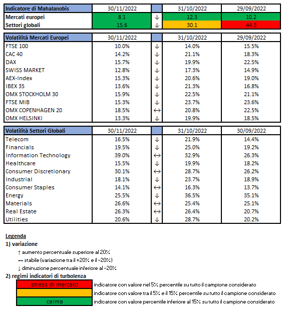
L’indicatore di Mahalanobis permette di evidenziare periodi di stress nei mercati finanziari. Si tratta di un indicatore che dipende dalle volatilità e dalle correlazioni di un particolare universo investimenti preso ad esame. Nello specifico ci siamo occupati dei mercati azionari europei e dei settori azionari globali.
Gli indici utilizzati sono:
Le volatilità riportate sono storiche e calcolate sugli ultimi 30 trading days disponibili. Per ogni asset-class dunque sono prima calcolati i rendimenti logaritmici dei prezzi degli indici di riferimento, successivamente si procede col calcolo della deviazione standard dei rendimenti, ed infine si procede a moltiplicare la deviazione standard per il fattore di annualizzazione.
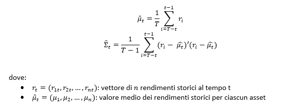
Per il calcolo della distanza di Mahalnobis si procede dapprima con la stima della matrice di covarianza tra le asset-class. Si considera l’approccio delle finestre mobili. Come con la volatilità, si procede prima con il calcolo dei rendimenti logaritmici e poi con la stima storica della matrice di covarianza, come riportato di seguito.
Supponendo una finestra mobile di T periodi, viene calcolato il valore medio e la matrice varianza covarianza al tempo t come segue:
La distanza di Mahalanobis è definita formalmente come:
Le parametrizzazioni che sono state scelte sono:
Rilevazioni mensili
Tempo T della finestra mobile pari a 5 anni (60 osservazioni mensili)
Le statistiche percentili sono state calcolate a partire dalla distribuzione dell’indicatore di Mahalanobis dal Dicembre 1997 al Dicembre 2019 su rilevazioni mensili.
Disclaimer: Le informazioni contenute in questa pagina sono esclusivamente a scopo informativo e per uso personale. Le informazioni possono essere modificate da finriskalert.it in qualsiasi momento e senza preavviso. Finriskalert.it non può fornire alcuna garanzia in merito all’affidabilità, completezza, esattezza ed attualità dei dati riportati e, pertanto, non assume alcuna responsabilità per qualsiasi danno legato all’uso, proprio o improprio delle informazioni contenute in questa pagina. I contenuti presenti in questa pagina non devono in alcun modo essere intesi come consigli finanziari, economici, giuridici, fiscali o di altra natura e nessuna decisione d’investimento o qualsiasi altra decisione deve essere presa unicamente sulla base di questi dati.
Questo sito utilizza cookie tecnici e di profilazione, propri e di terze parti, per garantire la corretta navigazione, analizzare il traffico e misurare l'efficacia delle attività di comunicazione.
Questo sito Web utilizza i cookie per migliorarne l'esperienza di navigazione. I cookie classificati come necessari, sono essenziali alle funzioni di base sito e vengono sempre memorizzati nel tuo browser. I cookie di terze parti, che ci aiutano ad analizzare e capire come utilizzi questo sito, vengono memorizzati nel tuo browser solo con il tuo consenso. Di seguito hai la possibilità di disattivare questi cookie. Tieni in conto che la disattivazione di alcuni di questi cookie potrebbe influire sulla tua esperienza di navigazione.
Necessary cookies are absolutely essential for the website to function properly. These cookies ensure basic functionalities and security features of the website, anonymously.
Cookie
Durata
Descrizione
cookielawinfo-checkbox-analytics
1 year
Cookie tecnico impostato dal plugin GDPR Cookie Consent che viene utilizzato per registrare il consenso dell'utente per i cookie nella categoria "Analitici".
cookielawinfo-checkbox-necessary
1 year
Cookie tecnico impostato dal plugin GDPR Cookie Consent che viene utilizzato per registrare il consenso dell'utente ai cookie.
CookieLawInfoConsent
1 year
Cookie tecnico impostato dal plugin GDPR Cookie Consent per salvare le scelte si/no dell'utente per ciascuna categoria.
viewed_cookie_policy
1 year
Cookie tecnico impostato dal plugin GDPR Cookie Consent che registra lo stato del pulsante predefinito della categoria corrispondente.
Analytical cookies are used to understand how visitors interact with the website. These cookies help provide information on metrics the number of visitors, bounce rate, traffic source, etc.
Cookie
Durata
Descrizione
_pk_id.gV3j99y0AE.0928
1 year 27 days
Cookie analitico impostato da Matomo e utilizzato per memorizzare alcuni dettagli sull'utente come l'ID univoco del visitatore
_pk_ses.gV3j99y0AE.0928
30 minutes
Cookie analitico impostato da Matomo di breve durata e utilizzato per memorizzare temporaneamente i dati della visita