Per 89 banche vigilate dalla BCE il coefficiente finale medio di CET1 nello scenario avverso su un orizzonte di tre anni è pari al 9,9%, 5,2 punti percentuali in meno rispetto al punto di partenza del 15,1%…
L’iniziativa di Finriskalert.it “Il termometro dei mercati finanziari” vuole presentare un indicatore settimanale sul grado di turbolenza/tensione dei mercati finanziari, con particolare attenzione all’Italia.
Significato degli indicatori
Rendimento borsa italiana: rendimento settimanale dell’indice della borsa italiana FTSEMIB;
Volatilità implicita borsa italiana: volatilità implicita calcolata considerando le opzioni at-the-money sul FTSEMIB a 3 mesi;
Future borsa italiana: valore del future sul FTSEMIB;
CDS principali banche 10Ysub: CDS medio delle obbligazioni subordinate a 10 anni delle principali banche italiane (Unicredit, Intesa San Paolo, MPS, Banco BPM);
Tasso di interesse ITA 2Y: tasso di interesse costruito sulla curva dei BTP con scadenza a due anni;
Spread ITA 10Y/2Y : differenza del tasso di interesse dei BTP a 10 anni e a 2 anni;
Rendimento borsa europea: rendimento settimanale dell’indice delle borse europee Eurostoxx;
Volatilità implicita borsa europea: volatilità implicita calcolata sulle opzioni at-the-money sull’indice Eurostoxx a scadenza 3 mesi;
Rendimento borsa ITA/Europa: differenza tra il rendimento settimanale della borsa italiana e quello delle borse europee, calcolato sugli indici FTSEMIB e Eurostoxx;
Spread ITA/GER: differenza tra i tassi di interesse italiani e tedeschi a 10 anni;
Spread EU/GER: differenza media tra i tassi di interesse dei principali paesi europei (Francia, Belgio, Spagna, Italia, Olanda) e quelli tedeschi a 10 anni;
Euro/dollaro: tasso di cambio euro/dollaro;
Spread US/GER 10Y: spread tra i tassi di interesse degli Stati Uniti e quelli tedeschi con scadenza 10 anni;
Prezzo Oro: quotazione dell’oro (in USD)
Spread 10Y/2Y Euro Swap Curve: differenza del tasso della curva EURO ZONE IRS 3M a 10Y e 2Y;
Euribor 6M: tasso euribor a 6 mesi.
I colori sono assegnati in un’ottica VaR: se il valore riportato è superiore (inferiore) al quantile al 15%, il colore utilizzato è l’arancione. Se il valore riportato è superiore (inferiore) al quantile al 5% il colore utilizzato è il rosso. La banda (verso l’alto o verso il basso) viene selezionata, a seconda dell’indicatore, nella direzione dell’instabilità del mercato. I quantili vengono ricostruiti prendendo la serie storica di un anno di osservazioni: ad esempio, un valore in una casella rossa significa che appartiene al 5% dei valori meno positivi riscontrati nell’ultimo anno. Per le prime tre voci della sezione “Politica Monetaria”, le bande per definire il colore sono simmetriche (valori in positivo e in negativo). I dati riportati provengono dal database Thomson Reuters. Infine, la tendenza mostra la dinamica in atto e viene rappresentata dalle frecce: ↑,↓, ↔ indicano rispettivamente miglioramento, peggioramento, stabilità rispetto alla rilevazione precedente.
Disclaimer: Le informazioni contenute in questa pagina sono esclusivamente a scopo informativo e per uso personale. Le informazioni possono essere modificate da finriskalert.it in qualsiasi momento e senza preavviso. Finriskalert.it non può fornire alcuna garanzia in merito all’affidabilità, completezza, esattezza ed attualità dei dati riportati e, pertanto, non assume alcuna responsabilità per qualsiasi danno legato all’uso, proprio o improprio delle informazioni contenute in questa pagina. I contenuti presenti in questa pagina non devono in alcun modo essere intesi come consigli finanziari, economici, giuridici, fiscali o di altra natura e nessuna decisione d’investimento o qualsiasi altra decisione deve essere presa unicamente sulla base di questi dati.
New Jersey, Texas, and Alabama have individual state regulators issuing concerns that New Jersey-based DeFi firm, BlockFi, is offering unregistered securities…
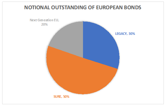
The EU is set to become the largest supranational bond issuer in the world thanks to its €90bn billion instrument for temporary Support to mitigate Unemployment Risks in an Emergency (SURE) and €750bn Next Generation EU (NGEU) recovery fund. If we look at the distribution of bond notional issued by the European Union outstanding as at the end of June and we divide it between SURE, NGEU and legacy programmes (mainly for loans to Ireland and Portugal during the last debt crisis) we can see that the SURE programme (now concluded) represents almost 50% of total with NGEU already representing 20%.
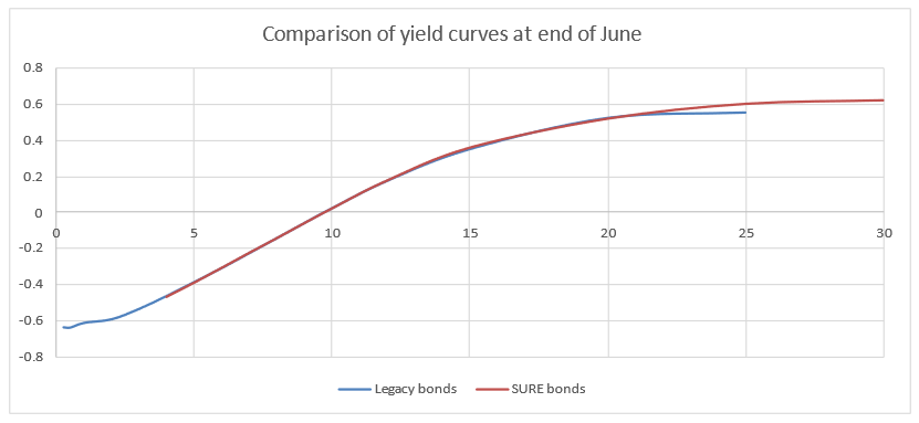
This significant amount of new bond issued on the market doesn’t present a material liquidity spread if we compare the Legacy vs the SURE yield structures.
Because of its material significance in terms of notional issued, we will analyse the financial aspect of the SURE programme in the rest of the article. The plans to mitigate Unemployment Risks in an Emergency financed through the SURE programme nor the social characteristics of the bonds issued will be part of an upcoming article.
The SURE instrument was created by the European Union (EU) to help Member States protect workers’ jobs and income during pandemic. It gave such a financial assistance in the form of loans with favourable conditions to the Member States. Each Member State benefitting from financial assistance under SURE was in fact required to sign a loan agreement with the Commission laying down the characteristics of the loan. Most of the loan agreements were signed in the third quarter of 2020, which enabled the Commission to issue SURE bonds starting from October 2020. The agreements guarantee that the loans between the Commission and the Member States are in back-to-back, meaning that the Commission borrows on behalf of the Union and then lends to Member States at the same conditions.
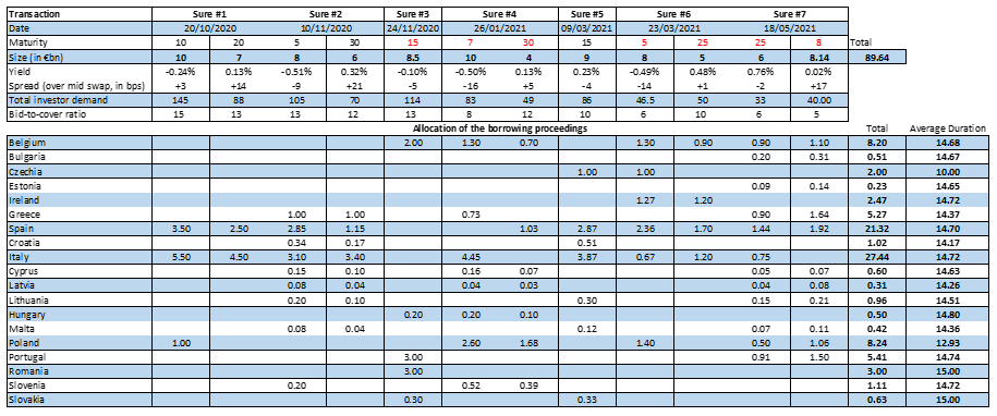
In the tables below we report the results of the Commission borrowing (table on the top) and how the proceedings have been distributed to the different member states.
From the table we can notice that:
The first SURE transaction represented largest ever order book (€233 billion) for any deal in the history of the global bond markets.
The major beneficiaries of the SURE program were Italy (€27.44bn) and Spain (€21.32bn) who have borrowed almost 55% of the total funds available
The average duration of the loans between each Member State and the European Commission is around 15 years with only Czechia having borrowed at 10 year
The countries whose debt trades at yields below the European Union one (eg. Germany, Austria, Netherlands) or the ones that have a very similar level of yields (eg. France) have not accessed the programme because it was not financially advantageous for them
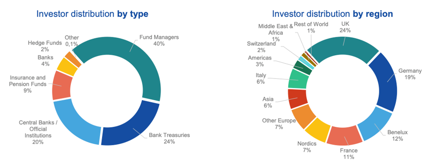
The bonds have attracted a significant of interest from the investors, especially for the first tranches: a very healthy average bid-to-cover ratios around 10 highlights the appetite for a AAA security that prices higher yields than Germany. The biggest majority of the investors where fund managers, as described in the graph below[1]
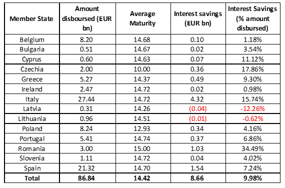
Because of the back-to-back lending structure, the loans disbursed under SURE generated interest rate savings for the vast majority of the Member States as the Commission was able to obtain favourable terms on the capital markets. To compute the savings, it is assumed that, in the absence of loans from SURE, Member States would have issued bonds with the same characteristics (i.e. maturity and coupon) as the EU SURE bonds on the day the loans were disbursed. The difference in yield between the government bond on the secondary market and the bond issued by the Commission is multiplied by the maturity of the bond and the notional of the back-to-back loan. We summarise the results of the analysis in the table below[2].
Here are the main takeaways from the table:
Italy saves the most interest rates (€4.32bn). This amount represents half of the total savings locked through the SURE financing project by all the Member States.
The country that saves the most interest rate as a percentage of the amount disbursed is Romania. This is because it received only a 15 year €3bn back-to-back loan. On the long maturities, total interest savings tend to be higher than the product of the average spread and the average maturity. The spread and the maturity are generally positively correlated, i.e. EU SURE yield curves tend to be flatter than national yield curves.
The Member States that benefited more from the SURE programme were Italy, Spain, Romania and Greece. Looking at the programme from this perspective evidences in a very effective way that this was first time a EU programme is directed not proportionally to the population of the and addresses the Countries most in need.
The SURE programme hence represents a win-win for the European Union (who has now established more firmly its presence on the capital markets) and the Member States (who have recorded significant interest rate gains). It paved the way to an instrument like the NGEU which is going to re-interpret the back-to-back lending structure in light of the new grants offered to Member States. “The successful SURE programme which served as a kind of test run makes us confident that the NGEU bonds will meet both our and the investors’ expectations” said Johannes Hahn, European Commissioner for Budget and Administration. We’ll analyse the NGEU programme in future articles.
[1] Source: European Commission – “Borrowing to finance the recovery: EU’s upcoming issuance under NGEU – Investor Call” – June 2021
[2] We have excluded from the analysis Estonia, Croatia, Hungary, Malta and Slovakia because of the limited size of the bonds issued. These represent less than 3bn of the total amount disbursed.
Questo sito utilizza cookie tecnici e di profilazione, propri e di terze parti, per garantire la corretta navigazione, analizzare il traffico e misurare l'efficacia delle attività di comunicazione.
Questo sito Web utilizza i cookie per migliorarne l'esperienza di navigazione. I cookie classificati come necessari, sono essenziali alle funzioni di base sito e vengono sempre memorizzati nel tuo browser. I cookie di terze parti, che ci aiutano ad analizzare e capire come utilizzi questo sito, vengono memorizzati nel tuo browser solo con il tuo consenso. Di seguito hai la possibilità di disattivare questi cookie. Tieni in conto che la disattivazione di alcuni di questi cookie potrebbe influire sulla tua esperienza di navigazione.
Necessary cookies are absolutely essential for the website to function properly. These cookies ensure basic functionalities and security features of the website, anonymously.
Cookie
Durata
Descrizione
cookielawinfo-checkbox-analytics
1 year
Cookie tecnico impostato dal plugin GDPR Cookie Consent che viene utilizzato per registrare il consenso dell'utente per i cookie nella categoria "Analitici".
cookielawinfo-checkbox-necessary
1 year
Cookie tecnico impostato dal plugin GDPR Cookie Consent che viene utilizzato per registrare il consenso dell'utente ai cookie.
CookieLawInfoConsent
1 year
Cookie tecnico impostato dal plugin GDPR Cookie Consent per salvare le scelte si/no dell'utente per ciascuna categoria.
viewed_cookie_policy
1 year
Cookie tecnico impostato dal plugin GDPR Cookie Consent che registra lo stato del pulsante predefinito della categoria corrispondente.
Analytical cookies are used to understand how visitors interact with the website. These cookies help provide information on metrics the number of visitors, bounce rate, traffic source, etc.
Cookie
Durata
Descrizione
_pk_id.gV3j99y0AE.0928
1 year 27 days
Cookie analitico impostato da Matomo e utilizzato per memorizzare alcuni dettagli sull'utente come l'ID univoco del visitatore
_pk_ses.gV3j99y0AE.0928
30 minutes
Cookie analitico impostato da Matomo di breve durata e utilizzato per memorizzare temporaneamente i dati della visita