Il lavoro valuta gli effetti macroeconomici nazionali e internazionali, nonché quelli sull’efficacia della politica monetaria, derivanti dall’introduzione di valute digitali…
Mag
06
2022
Il lavoro valuta gli effetti macroeconomici nazionali e internazionali, nonché quelli sull’efficacia della politica monetaria, derivanti dall’introduzione di valute digitali…

L’industria italiana dei minibond ha conquistato un rilevante numero di nuove emittenti nel 2021 e ha recuperato i livelli pre-Covid. Lo ‘certifica’ il nuovo Report dell’Osservatorio Minibond pubblicato dalla School of Management del Politecnico di Milano.
I minibond sono obbligazioni e cambiali finanziarie di importo inferiore a € 50 milioni emessi da società non finanziarie e rappresentano ormai da 10 anni un’opportunità di diversificazione delle fonti di finanziamento per le PMI e anche una ‘palestra’ per rapportarsi con il mercato mobiliare e con i fondi di investimento.
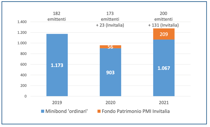
Nel 2021 il mercato italiano si è ripreso velocemente rispetto al 2020, anche grazie alle garanzie pubbliche potenziate a valle degli effetti della pandemia Covid-19. Nei 12 mesi si è registrato un controvalore raccolto pari a € 1,67 miliardi attraverso 219 emissioni, rispetto a € 900 milioni raccolti con 191 emissioni dell’anno precedente (si veda la Figura). Un’ulteriore spinta è arrivata dalla misura del Fondo Patrimonio PMI di Invitalia (che ha sostenuto attraverso la sottoscrizione di minibond a tasso agevolato le operazioni di patrimonializzazione attuate con equity dalle PMI), che solo nel 2021 ha coinvolto 131 imprese, per un controvalore di € 209 milioni.
Le imprese emittenti
Analizzando il mercato nel suo complesso, sono 832 le imprese italiane non finanziarie che alla data del 31 dicembre 2021 – a partire da novembre 2012 – hanno collocato minibond, di cui 520 PMI (il 62,5%). Solo nel 2021 le emittenti sono state 200 (di cui ben 163 si sono affacciate sul mercato per la prima volta), in aumento rispetto alle 173 del 2020: si tratta per il 52,0% di SpA, per il 45,0% di Srl e per il 3,0% di società cooperative. Per quanto riguarda il settore di attività, il comparto manifatturiero è in testa (41,5% del campione 2021), seguito dal commercio (14,0%), mentre la distribuzione geografica vede riconquistare il primo posto dalla Lombardia (45 emittenti), seguita da Campania (39) ed Emilia-Romagna (27).
Le emissioni
Le 219 emissioni del 2021 fanno registrare un valore medio tendenziale pari a € 4,75 milioni, nonostante il 43% dei collocamenti sia stato di importo inferiore a € 2 milioni. Solo una piccola parte dei titoli è stata quotata su un mercato borsistico (15%, di cui il 12% su ExtraMOT PRO3 e il 3% su un listino estero). Molto variegata continua ad essere la scadenza, con una serie di titoli short term con maturity a pochi mesi ed emissioni a più lunga scadenza, mentre per il rimborso l’opzione a rate successive (amortizing) è largamente preferita a quella bullet. Per quanto riguarda la cedola, nella maggioranza dei casi è fissa. Cresce leggermente la remunerazione (la media è 3,65% rispetto a 3,61% dell’anno prima) anche grazie a numerose emissioni che prevedono garanzie pubbliche. I titoli senza garanzie sono dunque una minoranza del mercato. La presenza di opzioni call e put rispetto al rimborso del capitale è frequente nei minibond; nel 2021 sono aumentati quelli che presentano l’opzione call di rimborso anticipato a discrezione dell’emittente.
Basket bond
Nel 2021 hanno acquisito ulteriore spazio i basket bond, ovvero progetti di sistema volti ad aggregare le emittenti per area geografica o per filiera produttiva, anche attraverso operazioni di cartolarizzazione. Questo tipo di operazioni è utile non solo a diversificare il rischio e raggiungere masse critiche interessanti per investitori che difficilmente guarderebbero al mondo dei minibond, ma anche per l’aspetto ‘educativo’ legato al coinvolgimento di più aziende che decidono di mettersi in gioco assieme. Fino ad oggi sono state contate 11 iniziative che hanno catalizzato oltre € 1,2 miliardi di risorse, in cui sia Cassa Depositi e Prestiti (CDP) sia il Fondo Europeo per gli Investimenti (FEI) hanno avuto un fondamentale ruolo di anchor investor.
Green minibond
La crescente attenzione del mercato finanziario verso la sostenibilità e i temi ESG sta alimentando le emissioni di green bond, titoli obbligazionari emessi per finanziare progetti con un impatto positivo in termini ambientali. Questo boom ha inevitabilmente influenzato anche il mercato italiano dei green minibond, praticamente inesistente fino al 2017. Dal 2018 al 2020 compaiono 9 titoli qualificabili come green, per una raccolta di € 125,8 milioni. Nel solo 2021 si registrano 14 collocamenti per un controvalore di € 77,85 milioni. Questo evidenzia non solo l’inizio di un ciclo favorevole, ma anche l’arrivo di emissioni di importo contenuto, destinate quindi a finanziare progetti di più piccola taglia rispetto al passato.
Gli investitori
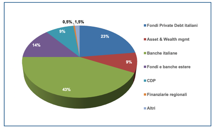
Per quanto riguarda gli investitori che hanno sottoscritto i minibond, il 2021 ha confermato il ruolo importante delle banche italiane (hanno sottoscritto il 43% dei volumi) seguite dai fondi di private debt (23%). Fondi e banche estere hanno contribuito con il 14%, mentre Cassa Depositi e Prestiti con il 9%. Ai numeri citati è possibile affiancare l’investimento di € 209 milioni che Invitalia ha sottoscritto nel 2021 nei minibond di Fondo Patrimonio PMI. Infine, seppur le banche e i fondi di credito abbiano fatto la parte del leone, la disciplina dei cosiddetti ‘PIR alternativi’ e la possibilità per i portali di equity crowdfunding autorizzati dalla Consob di collocare minibond attraverso una sezione dedicata della piattaforma, ha aperto la possibilità d’investimento dedicata – sotto alcune condizioni – anche a investitori non professionali.
Le prospettive future
Le tensioni geo-politiche che hanno influenzato i primi mesi del 2022 e la corrispondente impennata dei costi delle materie prime e dell’energia stanno avendo un impatto negativo sull’economia nazionale ed internazionale, rendendo difficile tracciare previsioni affidabili per l’anno corrente. Tuttavia, risulta ragionevole pensare che i nuovi programmi di basket bond, la crescente attenzione verso le tematiche ESG e iniziative come quella del Fondo Patrimonio PMI di Invitalia, possano generare per le aziende italiane nuove opportunità di raccolta di capitale attraverso minibond. Le aspettative sono quindi di una conferma dei numeri visti nel 2021.

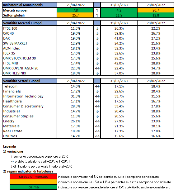
L’indicatore di Mahalanobis permette di evidenziare periodi di stress nei mercati finanziari. Si tratta di un indicatore che dipende dalle volatilità e dalle correlazioni di un particolare universo investimenti preso ad esame. Nello specifico ci siamo occupati dei mercati azionari europei e dei settori azionari globali.
Gli indici utilizzati sono:

Le volatilità riportate sono storiche e calcolate sugli ultimi 30 trading days disponibili. Per ogni asset-class dunque sono prima calcolati i rendimenti logaritmici dei prezzi degli indici di riferimento, successivamente si procede col calcolo della deviazione standard dei rendimenti, ed infine si procede a moltiplicare la deviazione standard per il fattore di annualizzazione.
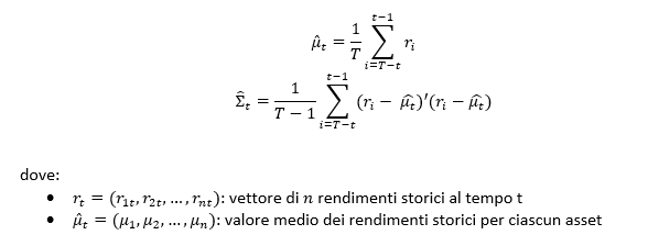
Per il calcolo della distanza di Mahalnobis si procede dapprima con la stima della matrice di covarianza tra le asset-class. Si considera l’approccio delle finestre mobili. Come con la volatilità, si procede prima con il calcolo dei rendimenti logaritmici e poi con la stima storica della matrice di covarianza, come riportato di seguito.
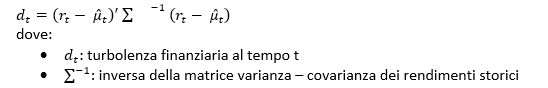
Supponendo una finestra mobile di T periodi, viene calcolato il valore medio e la matrice varianza covarianza al tempo t come segue:
La distanza di Mahalanobis è definita formalmente come:
Le parametrizzazioni che sono state scelte sono:
Le statistiche percentili sono state calcolate a partire dalla distribuzione dell’indicatore di Mahalanobis dal Dicembre 1997 al Dicembre 2019 su rilevazioni mensili.
Ulteriori dettagli sono riportati in questo articolo.
Disclaimer: Le informazioni contenute in questa pagina sono esclusivamente a scopo informativo e per uso personale. Le informazioni possono essere modificate da finriskalert.it in qualsiasi momento e senza preavviso. Finriskalert.it non può fornire alcuna garanzia in merito all’affidabilità, completezza, esattezza ed attualità dei dati riportati e, pertanto, non assume alcuna responsabilità per qualsiasi danno legato all’uso, proprio o improprio delle informazioni contenute in questa pagina. I contenuti presenti in questa pagina non devono in alcun modo essere intesi come consigli finanziari, economici, giuridici, fiscali o di altra natura e nessuna decisione d’investimento o qualsiasi altra decisione deve essere presa unicamente sulla base di questi dati.

L’iniziativa di Finriskalert.it “Il termometro dei mercati finanziari” vuole presentare un indicatore settimanale sul grado di turbolenza/tensione dei mercati finanziari, con particolare attenzione all’Italia.
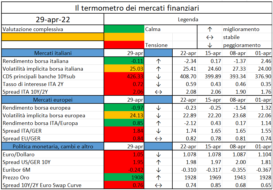
Significato degli indicatori
I colori sono assegnati in un’ottica VaR: se il valore riportato è superiore (inferiore) al quantile al 15%, il colore utilizzato è l’arancione. Se il valore riportato è superiore (inferiore) al quantile al 5% il colore utilizzato è il rosso. La banda (verso l’alto o verso il basso) viene selezionata, a seconda dell’indicatore, nella direzione dell’instabilità del mercato. I quantili vengono ricostruiti prendendo la serie storica di un anno di osservazioni: ad esempio, un valore in una casella rossa significa che appartiene al 5% dei valori meno positivi riscontrati nell’ultimo anno. Per le prime tre voci della sezione “Politica Monetaria”, le bande per definire il colore sono simmetriche (valori in positivo e in negativo). I dati riportati provengono dal database Thomson Reuters. Infine, la tendenza mostra la dinamica in atto e viene rappresentata dalle frecce: ↑,↓, ↔ indicano rispettivamente miglioramento, peggioramento, stabilità rispetto alla rilevazione precedente.
Disclaimer: Le informazioni contenute in questa pagina sono esclusivamente a scopo informativo e per uso personale. Le informazioni possono essere modificate da finriskalert.it in qualsiasi momento e senza preavviso. Finriskalert.it non può fornire alcuna garanzia in merito all’affidabilità, completezza, esattezza ed attualità dei dati riportati e, pertanto, non assume alcuna responsabilità per qualsiasi danno legato all’uso, proprio o improprio delle informazioni contenute in questa pagina. I contenuti presenti in questa pagina non devono in alcun modo essere intesi come consigli finanziari, economici, giuridici, fiscali o di altra natura e nessuna decisione d’investimento o qualsiasi altra decisione deve essere presa unicamente sulla base di questi dati.

Non è un momento facile per i banchieri centrali. Da un lato debbono occuparsi giorno per giorno di una tempesta perfetta (inflazione, rallentamento dell’economia, alto debito pubblico) dall’altra debbono gestire una svolta epocale quale l’introduzione della moneta di banca centrale digitale sotto la minaccia, per ora solo all’orizzonte, di monete digitali private, eventualmente promosse da qualche BigTech, o di monete digitali di qualche altro Stato.
Per chiarire di cosa stiamo parlando, la moneta di banca centrale digitale sarebbe l’equivalente delle banconote ma in forma digitale (esisterebbe soltanto nella rete). Avrebbe la solidità delle banconote in quanto il suo valore è garantito dalla Banca Centrale – e non sta quindi nei bilanci di una banca – e potrebbe essere utilizzata per fare i pagamenti online al posto dei bonifici bancari, delle carte di credito o di debito.
Curiosamente, ma non troppo, i paesi che rappresentano il cuore del sistema finanziario (Stati Uniti, Europa su tutti) procedono con i piedi di piombo valutando attentamente benefici e controindicazioni per il funzionamento e la stabilità del sistema finanziario e dell’economia reale. In Europa, complice anche la difficoltà di mettere d’accordo paesi che hanno diverse priorità, si stima che ci vorranno quattro anni per avere l’euro digitale nelle nostre tasche. La ragione di tutta questa cautela risiede nel fatto che la sua introduzione potrebbe cambiare radicalmente gli equilibri del sistema finanziario, in particolare potremmo avere una disintermediazione delle banche che avrebbero meno depositi nei loro bilanci con un conseguente aumento del costo del credito. Invece i paesi emergenti corrono. La Bank for International Settlements ha condotto una indagine su ventisei paesi emergenti circa le loro attività in merito, solo due paesi non prevedono di emettere moneta digitale in un prossimo futuro, diversi paesi – soprattutto in medio oriente e in Asia – sono invece in fase avanzata con lo sviluppo di progetti pilota. Un caso eclatante è rappresentato dalla Banca Centrale delle Bahamas che ha reso disponibile la sua moneta digitale (Sand dollar) al pubblico nell’ottobre 2020.
I motivi per progettare di emettere moneta digitale nei paesi emergenti sono più d’uno. In primo luogo l’utilizzo del contante sta diminuendo e al contempo i pagamenti digitali, che passano tramite sistemi privati (come le carte di credito o le app) stanno aumentando, questo potrebbe portare ad una perdita di centralità della Banca centrale nel gestire gli aggregati monetari e, quindi, nel controllare l’economia. Il secondo motivo è che una moneta digitale favorirebbe l’inclusione di larga parte della popolazione nel mondo finanziario. Si stima che circa 1/3 della popolazione adulta nel mondo non possieda un conto bancario, la percentuale supera il 50% in Africa e il 40% in America Latina ma molte di queste persone possiedono un telefono cellulare e sono quindi in grado di effettuare pagamenti digitali. Una moneta digitale unita ad una campagna per diminuire il digital divide potrebbe avvicinare parte della popolazione al mondo della finanza. Strettamente legata a questa considerazione abbiamo una terza ragione che riguarda i costi dei servizi di pagamento che sono molto elevati in questi paesi, una moneta di banca centrale potrebbe aumentare la competizione e l’efficienza nel settore del sistema dei pagamenti riducendone i costi.
Tra i principali punti di attenzione da parte delle banche centrali troviamo: problemi operativi, disintermediazione, basso livello di adozione. Il primo è quello che desta più preoccupazione sia riguardo a interruzioni del funzionamento dell’infrastruttura (rischio operativo), come si è verificato a gennaio nel caso del progetto pilota dell’Eastern Caribean Central Bank, sia per rischi di attacchi cyber. Il tema della disintermediazione delle banche, che potrebbe riflettersi in una riduzione del credito all’economia, è al centro dell’attenzione soprattutto per i suoi effetti nei periodi di crisi. Per fronteggiare il problema si ipotizza di porre un limite alla quantità di moneta digitale posseduta. Quanto all’adozione, il tema è quello di disegnare la moneta digitale in modo tale che venga adottata da una vasta platea di cittadini e imprese.
L’esperienza sul campo dei paesi emergenti permette di comprendere anche la piega che sta prendendo il disegno delle moneta digitale contribuendo a sgombrare un campo che rischia di essere troppo affollato da ipotesi e obiettivi da raggiungere.
In primo luogo, quasi tutti gli esperimenti vanno nella direzione di un sistema a due livelli con la banca centrale che fornisce l’infrastruttura ed emette la moneta mentre le banche si occupano dell’interfaccia con l’utente. E’ escluso quindi che la banca centrale faccia da banca direttamente per i cittadini.
Sul fronte dell’anonimato della moneta digitale ancora non c’è una chiara direzione. I pagamenti in contante sono anonimi a differenza di quelli effettuati tramite i circuiti bancari. Se le transazioni con moneta digitale debbono rispecchiare questa caratteristica è ancora una questione aperta anche se la Cina – ma anche le Bahamas – sembra segnare la via optando per mantenere l’anonimato per transazioni di valore limitato e piena tracciabilità per operazioni di ammontare significativo. Sul fronte dell’architetture (centralizzata o decentralizzata tramite una blockchain) così come sulla presenza di limiti alla detenzione della moneta digitale non c’è ancora una chiara scelta di campo anche se è probabile che qualche forma di limitazione alla detenzione di moneta digitale venga introdotta per limitare l’eventuale disintermediazione bancaria.
La priorità sembra essere quella di garantire l’interoperabilità della moneta digitale con altri sistemi di pagamento privati (la possibilità di convertire moneta digitale con moneta depositata presso conti correnti o utilizzata tramite altri sistemi), un aspetto tecnico che può segnare il successo dell’esperimento e che presenta più di una difficoltà. Un altro aspetto che emerge dall’esperienza sul campo è che le banche centrale sembrano voler non complicarsi troppo la vita non prevedendo una remunerazione della moneta digitale. Così facendo la moneta digitale sarebbe prossima al contante e non sarebbe destinata a fare concorrenza ai depositi.
Al fine di favorire l’inclusione finanziaria, le esperienze delle banche centrali nei paesi emergenti mostrano che alcune caratteristiche del disegno della moneta digitale potrebbero essere cruciali: disponibilità della moneta off-line, compatibilità con telefoni cellulari non di ultima generazione, basso costo rispetto a strumenti di pagamento alternativi, possibilità di effettuare l’on-boarding dell’utilizzatore online.
La sperimentazione in materia di moneta digitale va avanti, il terreno inizia a dissodarsi e a sgombrarsi delle diverse ipotesi sul terreno, la speranza è che l’Europa (o meglio i paesi dell’area dell’Euro) faccia tesoro di questa esperienza e non arrivi troppo tardi.
Il regolamento UE/2014/600 (MiFIR), entrato in vigore il 3 gennaio 2018, ha attribuito alle autorità di vigilanza nazionali, e in alcuni casi all’ESMA e all’EBA, il potere di vietare o limitare…
Introductory remarks by Luis de Guindos, Vice-President of the ECB, at the ECON Committee of the European Parliament
https://www.ecb.europa.eu//press/key/date/2022/html/ecb.sp220428~4e38b8ed52.en.html
Speech by Fabio Panetta, Member of the Executive Board of the ECB, at Columbia University…
https://www.ecb.europa.eu//press/key/date/2022/html/ecb.sp220425~6436006db0.en.html
