

Il termometro dei mercati finanziari (8 Aprile 2022)
a cura di Emilio Barucci e Daniele Marazzina

Apr 09 2022
Il termometro dei mercati finanziari (8 Aprile 2022)a cura di Emilio Barucci e Daniele Marazzina

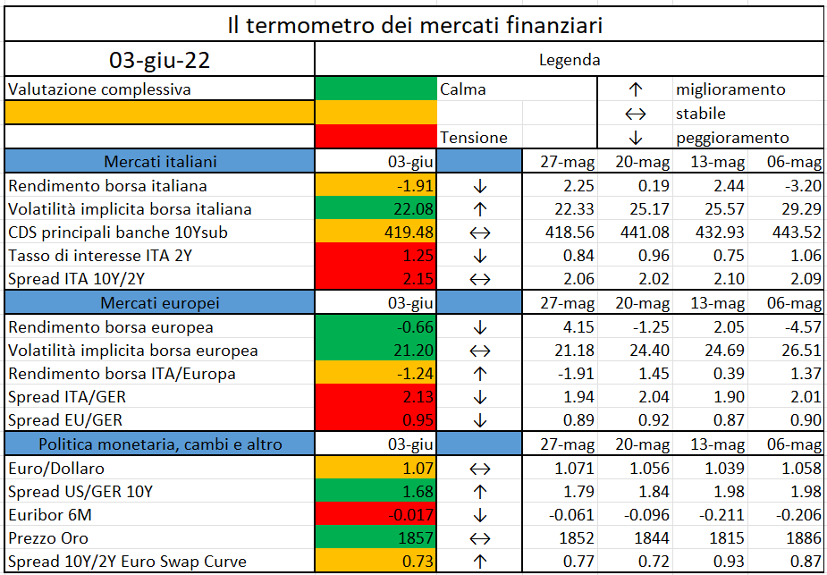
L’iniziativa di Finriskalert.it “Il termometro dei mercati finanziari” vuole presentare un indicatore settimanale sul grado di turbolenza/tensione dei mercati finanziari, con particolare attenzione all’Italia.
Significato degli indicatori

  • Rendimento borsa italiana: rendimento settimanale dell’indice della borsa italiana FTSEMIB;
  • Volatilità implicita borsa italiana: volatilità implicita calcolata considerando le opzioni at-the-money sul FTSEMIB a 3 mesi;
  • Future borsa italiana: valore del future sul FTSEMIB;
  • CDS principali banche 10Ysub: CDS medio delle obbligazioni subordinate a 10 anni delle principali banche italiane (Unicredit, Intesa San Paolo, MPS, Banco BPM);
  • Tasso di interesse ITA 2Y: tasso di interesse costruito sulla curva dei BTP con scadenza a due anni;
  • Spread ITA 10Y/2Y : differenza del tasso di interesse dei BTP a 10 anni e a 2 anni;
  • Rendimento borsa europea: rendimento settimanale dell’indice delle borse europee Eurostoxx;
  • Volatilità implicita borsa europea: volatilità implicita calcolata sulle opzioni at-the-money sull’indice Eurostoxx a scadenza 3 mesi;
  • Rendimento borsa ITA/Europa: differenza tra il rendimento settimanale della borsa italiana e quello delle borse europee, calcolato sugli indici FTSEMIB e Eurostoxx;
  • Spread ITA/GER: differenza tra i tassi di interesse italiani e tedeschi a 10 anni;
  • Spread EU/GER: differenza media tra i tassi di interesse dei principali paesi europei (Francia, Belgio, Spagna, Italia, Olanda) e quelli tedeschi a 10 anni;
  • Euro/dollaro: tasso di cambio euro/dollaro;
  • Spread US/GER 10Y: spread tra i tassi di interesse degli Stati Uniti e quelli tedeschi con scadenza 10 anni;
  • Prezzo Oro: quotazione dell’oro (in USD)
  • Spread 10Y/2Y Euro Swap Curve: differenza del tasso della curva EURO ZONE IRS 3M a 10Y e 2Y;
  • Euribor 6M: tasso euribor a 6 mesi.

I colori sono assegnati in un’ottica VaR: se il valore riportato è superiore (inferiore) al quantile al 15%, il colore utilizzato è l’arancione. Se il valore riportato è superiore (inferiore) al quantile al 5% il colore utilizzato è il rosso. La banda (verso l’alto o verso il basso) viene selezionata, a seconda dell’indicatore, nella direzione dell’instabilità del mercato. I quantili vengono ricostruiti prendendo la serie storica di un anno di osservazioni: ad esempio, un valore in una casella rossa significa che appartiene al 5% dei valori meno positivi riscontrati nell’ultimo anno. Per le prime tre voci della sezione “Politica Monetaria”, le bande per definire il colore sono simmetriche (valori in positivo e in negativo). I dati riportati provengono dal database Thomson Reuters. Infine, la tendenza mostra la dinamica in atto e viene rappresentata dalle frecce: ↑,↓, ↔  indicano rispettivamente miglioramento, peggioramento, stabilità rispetto alla rilevazione precedente.

Disclaimer: Le informazioni contenute in questa pagina sono esclusivamente a scopo informativo e per uso personale. Le informazioni possono essere modificate da finriskalert.it in qualsiasi momento e senza preavviso. Finriskalert.it non può fornire alcuna garanzia in merito all’affidabilità, completezza, esattezza ed attualità dei dati riportati e, pertanto, non assume alcuna responsabilità per qualsiasi danno legato all’uso, proprio o improprio delle informazioni contenute in questa pagina. I contenuti presenti in questa pagina non devono in alcun modo essere intesi come consigli finanziari, economici, giuridici, fiscali o di altra natura e nessuna decisione d’investimento o qualsiasi altra decisione deve essere presa unicamente sulla base di questi dati.

IFRS17 Bow Wave effect and Illiquidity Premium
a cura di Silvia Dell’Acqua

Apr 09 2022
IFRS17 Bow Wave effect and Illiquidity Premium a cura di Silvia Dell’Acqua

Following the overview provided in [5] “IFRS17 is coming soon”, this article focuses on a potential definition of Illiquidity Premium (IP) that appears to soften the so-called Bow Wave effect. Given a single value of IP, the author presents an alternative application to the risk-free rates other than the parallel shift, that reduces the gap between Real World and Risk Neutral evaluations, without introducing any bias: a mathematical and graphical proof is provided to show the equality of capitalization of the underlying volumes of reserves, that always reach the same value.

IFRS17 takes a longer-term view than IFRS4, immediately covering all the losses and postponing the profit profile, with this second feature driven by an unintended effect known as “Bow Wave”. For contracts where the VFA is used, the Bow Wave effect raises from the impact of Real Word (RW) returns on the unlocking of the Contractual Service Margin (CSM) in Risk Neutral (RN) projections.

The CSM is determined at initial recognition as the expected unearned profit embedded in the insurance contracts, based on an interest rate curve called locked in curve; the “unlocking of the CSM” indicates the adjustments applied to its value from time to time to offset the impacts of changes in the FCFs (Fulfilment Cash Flows) related to future services. The new accounting standards foresee that the CSM is amortized over the life of the contract and released into the P&L to best reflect the services already provided and the remaining duration: part of the CSM shall be released from reporting period to reporting period by considering the difference between the actual and expected service provided in the current period together with the expected service estimated for future periods, following an amortization pattern defined by the CU (Coverage Unit), that should represent a measure for the service delivery.

In a RN projection, on average, nothing can be earned more than the risk-free rate, however, in the RW, insurers expect to earn some excess of interest, often called “risk premium” or “expected spread”. If this “over-return” exists (it is positive), the IFRS17 principles state that the part belonging to the SH (Share Holder) shall be added to the CSM and released over the remaining duration. When the over-returns are systematic, the adjustments lead to a delay in the profit recognition, cumulate over time and, figuratively[1] speaking, generate a “Bow Wave” (BW) of excess of interests. A systematic delay of profits is not in line with the purpose of IFRS17, but, unfortunately, no patches have been hinted yet by either the standards or the IASB, albeit a solution must be found. Avoiding the BW effect means, in other words, having a release of CSM comparable with the one of a hypothetical CSM defined at inception and embedding all the future expected over-returns. This can be achieved in three possible ways (that can be potentially combined):

  • proper Illiquidity Premium

the idea is to define an IP that pushes the RN projection towards the RW one

  • CSM adjustment

the idea is to increase the CSM release by the SH share of excess of investment returns

  • modified CU

the idea is to consider the over return in the definition of CU

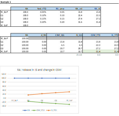
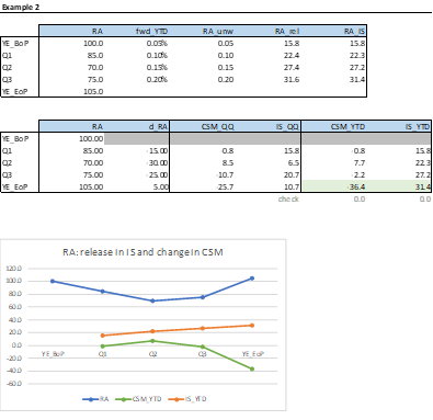
When [B] or [C] are chosen, the insurer should derive both the difference between the distribution of RW and RN returns in relation to the result of the reporting period (considering all the different asset classes, such as government and corporate bonds, equity, real estate, other investments) and the portion belonging to the SH (the SH share). In case of [B], the adjustment to the CSM can be either calculated by adopting a simplified approach, where the RW over-return of the investments is multiplied by a share derived from the experience, or by comparing the PVFP (Present Value of Future Profits) of two simulations, respectively run under the RN and RW measures. The table below provides an illustrative example of the CSM release, adopting, one at a time, the solutions outlined above, in different possible scenarios. 

The Author believes that [A], compared to [B] and [C], provides a (at least partial) cleaner solution to the problem, avoiding further adjustments to the CSM release. A possible implementation is discussed in the following.

As stated by the principles, the discount rates adopted to determine the FCFs shall both reflect the level of current interest rates and the illiquidity characteristic of the liabilities, to counterbalance the credit effect on the asset side. The discount rates can be defined following a bottom-up or top-down approach, that should lead to the same result: in case of spike in the credit spreads, the former would raise the risk-free yields by a proportionate Illiquidity Premium (IP) and the latter would decrease the portfolio yields by a portion of the credit risk. Under the bottom-up approach, an IP is added to the risk-free rate to reflect the illiquidity characteristics of the insurance contracts; under the top-down approach, the full market value yield on the relevant assets is deducted by its credit risk component, without deduction in respect of its illiquidity component. In theory, both methods should be equal. Indeed, by indicating with

the spread of a corporate bond (i.e. the difference between its yield and the risk free one) is given by

and, rearranging the terms, we have

or, in other words

top-down approach = bottom-up approach

IFRS17 is a principles-based standard, that sets out a guidance, without explicitly establishing the rules for discounting: to define their own approach, insurers can consider various possibilities, adopt a relevant judgment, and agree with their auditors. Albeit no formulas are indicated, let us recall paragraph 36, that describes how to define the discount rates, that shall:

  1. reflect the time value of money, the characteristics of the cash flows and the liquidity characteristics of the insurance contracts
  2. be consistent with observable current market prices for financial instruments with cash flows whose characteristics are consistent with those of the insurance contracts, in terms of, for example, timing, currency and liquidity
  3. exclude the effect of factors that influence such observable market prices but do not affect the future cash flows of the insurance contracts.

The Liquidity usually indicates the ease with which assets can be converted into cash without affecting their market price, being the cash the most liquid asset (it can be traded to buy anything). A feature that influences the liquidity of Liabilities is the change in their duration when stressed events occur: the more sensitive the duration is to stressed scenarios (such as a mass lapse), the more liquid is the contract (indeed UL products are more liquid than SAV ones). The comparison between the durations of the liabilities and the assets backing the liabilities can provide an indication of the share of the assets IP that can be applied to the liabilities. This share is referred to as the Application Ratio (AR).

Paragraph B79 introduces a guidance on how to assess the liquidity of insurance contracts by considering the features of the products, that can generate an exit-value, an inherent value, and an exit cost, all these three components influencing the liquidity of the product:

Yield curves reflect assets traded in active markets that the holder can typically sell readily at any time without incurring significant costs. In contrast, under some insurance contracts the entity cannot be forced to make payments earlier than the occurrence of insured events, or dates specified in the contracts.

Some examples are provided in the following

This view is aligned to what EIOPA has proposed in its consultation paper [3], when defining the degree of liquidity based on the terms and conditions of insurance contracts

A similar idea is also shared by the MCEV (Market Consistent Embedded Value): the principles state that “A liability is liquid if the liability cash flows are not reasonably predictable”. When a liability is illiquid (liquid), the corresponding cash flows are (not) predictable, and the insurance company is (not) willing to hold the backing assets to maturity to target a higher investment return, given by the risk-free rates plus a liquidity premium. When a “buy to hold” strategy is adopted, the insurer is not exposed to volatility of market prices and can therefore lock in the premium above the risk-free rate, that compensates the holder for locking up the investment for a long-term.

Finally, paragraphs B78-B85 highlight the key principles to follow for determining the liquidity premium:

  1. Maximize the use of observable inputs
  2. Reflect current market conditions
  3. Exercise judgment to assess the degree of similarity between the features of the insurance contracts and assets with observable prices and make further adjustments as needed

and paragraphs B78-B79 stress that discount rates shall exclude the credit risk, which is not a characteristic of the insurance contracts.

Therefore, to define the discount rate of the liabilities under the bottom-up approach, insures should

  • derive an IP based on the portfolio of assets held (removing the credit risk)
  • derive an AR either based on “buckets of illiquidity”, identified by the features of the products, or based on the level of assets and liabilities mismatch (duration gap)
  • define the discount rate as

Albeit, theoretically, highly illiquid insurance contracts may be distinguished by rates of discount higher than the expected yield of the backing (less illiquid) assets, the AR is usually capped at 100%, to avoid this to happen.  A sensible definition of AR may be

with dur_x indicating the duration of Assets (A) and Liabilities (L).

The bottom-up approach reminds the definition of the risk-free rates provided by EIOPA in the SII context, with the IP being like the VA (Volatility Adjustment), calibrated on the undertakings portfolios, rather than on an average European one and 65% being the AP. Such derivation would lead to a relatively small value of IP, comparable to the EIOPA VA, that would not solve the need of having a sensible RW CSM release.

The reason for that is the definition itself of the “gross” VA (i.e. before the application ratio), that is given by the sum of a government and corporate risk corrected spread components, with weights usually biased towards the first one, where the Risk Correction (RC) levels down or even exceeds the original spread. The RC is almost the same for all the portfolios, whether these belong to EIOPA or the entity, being defined over averages value of 30 years of history. An illustrative example is provided in the following table, where the EIOPA reference portfolio is compared to three illustrative entity specific portfolios

Such values are too low and do not reflect the liquidity of the liabilities at all. The Author believes there must be positive a correlation between the IP value and the Minimum Guaranteed rate offered by products; in fact, given the low level of interest rates the market is currently experiencing, insurance entities often invest in illiquid asset classes that can bridge the gap left behind by the fixed interest bonds, still satisfying the required level of cash flow matching. As a recap

  • the IP measures the premium of illiquidity of the liabilities
  • it cannot be measured over the liabilities, but it could be measured over a replicating portfolio of assets, that should exactly match the liabilities cash flows (even if it is common practice to look at the duration only)
  • the assets baking the liabilities are a good compromise and the author believes that the IP shall be derived for alternative assets too, by means of the look through, as they are used to match the liability cash flows: high level of minimum guaranteed returns would not be sustained by investing in government and corporate bonds only with a reasonable duration. At the end of the day, a private debt can be comparable to a bond, with the difference that the money is lent to a firm not quoted in the regulated markets: there is for sure a credit risk to be removed, but the remaining IP will be quite high. The IP will then be the asset spread deducted of its risky component and it can be identified as the bid-offer spread.

The following charts compares the net flows of three illustrative types of portfolios

  1. guaranteed return of 4% and a duration of 10.6 years
  2. guaranteed return of 0% and a duration of 6.3 years (lower IP expected)
  3. guaranteed return of 0% and recurrent premiums, with the same duration as the first one, 10.5 years, that should be as liquid as the second one

Despite having the same duration, the former and the latter portfolios are very different, with a) being highly illiquid, as few people would be willing to buy it, unless reducing its cost by including a premium for its illiquidity. In terms of cash flows, to replicate a) the company should hold assets at high yields, while c) can be managed with recurrent premiums and plain bonds.

Having defined the AR to apply to the IP, and the perimeter of assets from where it is derived, the Author presents its opinion on how the  

can be added to the risk-free rates to reduce the BW effect. The Bow Wave tends to hit more in the first years of projections, when the risk-free rates are negative and the RW return is positive. The idea behind this approach is to increase as much as possible the coherency between the RN capitalization and discount of the volumes projected, where the capitalization applies a yield of the Segregated Funds (r_SF) that is comparable to a RW value, as it still embeds the Unrealized Gains and Losses (UGL), albeit being RN. The solution is to define an IP that changes over time, following the pattern of the UGL. Let us indicate with

The IP to apply to the risk-free rates is given by

The following charts show graphically the idea behind the formulas: the total value of single IP that would be applied as a parallel shift to the risk-free curve over time is preserved and, instead of being flat, is split into a flat and UGL component. Three illustrative portfolios are compared, with a total IP of respectively 10bps (PTF_1), 30bps (PTF_2) and 50bps (PTF_3), and the parameters p_flat and scaling_max respectively set to 50% and 200%.

The two following charts clarify the decomposition of IP: in the former, the net single IP (red line) is applied as a parallel shift to the risk-free rates (the integral is given by the area of the rectangle), while, in the latter, the net IP (red area) is given by the sum of the two components (yellow, flat, and green, UGL), where the two areas equals those of the first chart, but the green one has a shape coherent to the UGL release. The total red area is the same by construction.

This graph shows the UGL value over time (blue line), compared to its average value (orange line), where they have both been normalized such that the average value equals 100%, to easily understand the application of scaling_max  and the definition of the green area. The amount of UGL is not of interest, just their release shape is

The following charts show some sensitivity analyses carried out on PTF_3 to outline the behavior of the final IP depending on the choice of the parameters p_flat  and scaling_max:   equal to 100% (or 0%) implies that no (or all) the UGL shape drives the IP application, scaling_max equal to 1000% (or 0%) describes a situation where no correction on the UGL release (or no UGL at all) is considered to define the final IP

Some comments:

  • the orange line (100%_200%, all flat) shows the starting point, where the IP application is coherent to the SII framework, where the VA is applied as a parallel shift to all the maturities
  • the light blue line (0%_0%, all UGL with no possibility of considering any because of the cap) reverts to the orange one. They are not the same as the UGL exist till year 19, while the LLP start at year 20. The integral of 20 years is spread over just 19 years
  • the blue line (50%_200%) is a meaningful choice in the author’s view
  • the grey line (0%, 200%) is steeper than the blue line allocating to the UGL component all the area at disposal
  • the yellow line (0%, 1000%) compares to the grey one, where the implication of not having any cap is shown: the UGL are massively released in the first years. It is also traces over the UGL release shape outlined above.

This final chart provides a proof of the convergency of the capitalization under these very different cases: the capitalization value is preserved as the integral is. This is the proof that the approach does not introduce any bias as no additional source of illiquidity premium is added: the total value is just spread out in a more sensible way, reducing the Bow Wave effect.

Reference:

[1] IFRS – IFRS17 Insurance Contracts and Amendments to IFRS17, May 2017 and following

[2] IFRS – Transition Resource Group for IFRS 17 Insurance Contracts, September 2018

[3] EIOPA – Technical specification of the information request on the 2020 review of SII, March 2020

[4] DAV – IFRS 17 for German life insurance, May 2020

[5] Silvia D.A., Annalisa Iacobone – IFRS17 is coming soon, November 2021


[1] A bow wave is the progressive disturbance propagated through the water because of the displacement by the foremost point of the ship, the bow, that moves faster than the waves. It defines the wake of the ship, that, view from above, is V-shaped.

Indice di turbolenza dei mercati (31 Marzo 2022)
a cura di Gianni Pola e Antonello Avino

Apr 03 2022
Indice di turbolenza dei mercati (31 Marzo 2022)a cura di Gianni Pola e Antonello Avino

L’indicatore di Mahalanobis permette di evidenziare periodi di stress nei mercati finanziari. Si tratta di un indicatore che dipende dalle volatilità e dalle correlazioni di un particolare universo investimenti preso ad esame. Nello specifico ci siamo occupati dei mercati azionari europei e dei settori azionari globali.

Gli indici utilizzati sono:

Questa immagine ha l'attributo alt vuoto; il nome del file è Immagine-4.png

Le volatilità riportate sono storiche e calcolate sugli ultimi 30 trading days disponibili. Per ogni asset-class dunque sono prima calcolati i rendimenti logaritmici dei prezzi degli indici di riferimento, successivamente si procede col calcolo della deviazione standard dei rendimenti, ed infine si procede a moltiplicare la deviazione standard per il fattore di annualizzazione.

Per il calcolo della distanza di Mahalnobis si procede dapprima con la stima della matrice di covarianza tra le asset-class. Si considera l’approccio delle finestre mobili. Come con la volatilità, si procede prima con il calcolo dei rendimenti logaritmici e poi con la stima storica della matrice di covarianza, come riportato di seguito.

Supponendo una finestra mobile di  T periodi, viene calcolato il valore medio e la matrice varianza covarianza al tempo t come segue:

Questa immagine ha l'attributo alt vuoto; il nome del file è image-6.png

La distanza di Mahalanobis è definita formalmente come:

Questa immagine ha l'attributo alt vuoto; il nome del file è image-7.png

Le parametrizzazioni che sono state scelte sono:

  • Rilevazioni mensili
  • Tempo T della finestra mobile pari a 5 anni (60 osservazioni mensili)

Le statistiche percentili sono state calcolate a partire dalla distribuzione dell’indicatore di Mahalanobis dal Dicembre 1997 al Dicembre 2019 su rilevazioni mensili.

Ulteriori dettagli sono riportati in questo articolo.

Disclaimer: Le informazioni contenute in questa pagina sono esclusivamente a scopo informativo e per uso personale. Le informazioni possono essere modificate da finriskalert.it in qualsiasi momento e senza preavviso. Finriskalert.it non può fornire alcuna garanzia in merito all’affidabilità, completezza, esattezza ed attualità dei dati riportati e, pertanto, non assume alcuna responsabilità per qualsiasi danno legato all’uso, proprio o improprio delle informazioni contenute in questa pagina. I contenuti presenti in questa pagina non devono in alcun modo essere intesi come consigli finanziari, economici, giuridici, fiscali o di altra natura e nessuna decisione d’investimento o qualsiasi altra decisione deve essere presa unicamente sulla base di questi dati.

Il termometro dei mercati finanziari (1 Aprile 2022)
a cura di Emilio Barucci e Daniele Marazzina

Apr 03 2022
Il termometro dei mercati finanziari (1 Aprile 2022)a cura di Emilio Barucci e Daniele Marazzina

L’iniziativa di Finriskalert.it “Il termometro dei mercati finanziari” vuole presentare un indicatore settimanale sul grado di turbolenza/tensione dei mercati finanziari, con particolare attenzione all’Italia.

Significato degli indicatori

  • Rendimento borsa italiana: rendimento settimanale dell’indice della borsa italiana FTSEMIB;
  • Volatilità implicita borsa italiana: volatilità implicita calcolata considerando le opzioni at-the-money sul FTSEMIB a 3 mesi;
  • Future borsa italiana: valore del future sul FTSEMIB;
  • CDS principali banche 10Ysub: CDS medio delle obbligazioni subordinate a 10 anni delle principali banche italiane (Unicredit, Intesa San Paolo, MPS, Banco BPM);
  • Tasso di interesse ITA 2Y: tasso di interesse costruito sulla curva dei BTP con scadenza a due anni;
  • Spread ITA 10Y/2Y : differenza del tasso di interesse dei BTP a 10 anni e a 2 anni;
  • Rendimento borsa europea: rendimento settimanale dell’indice delle borse europee Eurostoxx;
  • Volatilità implicita borsa europea: volatilità implicita calcolata sulle opzioni at-the-money sull’indice Eurostoxx a scadenza 3 mesi;
  • Rendimento borsa ITA/Europa: differenza tra il rendimento settimanale della borsa italiana e quello delle borse europee, calcolato sugli indici FTSEMIB e Eurostoxx;
  • Spread ITA/GER: differenza tra i tassi di interesse italiani e tedeschi a 10 anni;
  • Spread EU/GER: differenza media tra i tassi di interesse dei principali paesi europei (Francia, Belgio, Spagna, Italia, Olanda) e quelli tedeschi a 10 anni;
  • Euro/dollaro: tasso di cambio euro/dollaro;
  • Spread US/GER 10Y: spread tra i tassi di interesse degli Stati Uniti e quelli tedeschi con scadenza 10 anni;
  • Prezzo Oro: quotazione dell’oro (in USD)
  • Spread 10Y/2Y Euro Swap Curve: differenza del tasso della curva EURO ZONE IRS 3M a 10Y e 2Y;
  • Euribor 6M: tasso euribor a 6 mesi.

I colori sono assegnati in un’ottica VaR: se il valore riportato è superiore (inferiore) al quantile al 15%, il colore utilizzato è l’arancione. Se il valore riportato è superiore (inferiore) al quantile al 5% il colore utilizzato è il rosso. La banda (verso l’alto o verso il basso) viene selezionata, a seconda dell’indicatore, nella direzione dell’instabilità del mercato. I quantili vengono ricostruiti prendendo la serie storica di un anno di osservazioni: ad esempio, un valore in una casella rossa significa che appartiene al 5% dei valori meno positivi riscontrati nell’ultimo anno. Per le prime tre voci della sezione “Politica Monetaria”, le bande per definire il colore sono simmetriche (valori in positivo e in negativo). I dati riportati provengono dal database Thomson Reuters. Infine, la tendenza mostra la dinamica in atto e viene rappresentata dalle frecce: ↑,↓, ↔  indicano rispettivamente miglioramento, peggioramento, stabilità rispetto alla rilevazione precedente.

Disclaimer: Le informazioni contenute in questa pagina sono esclusivamente a scopo informativo e per uso personale. Le informazioni possono essere modificate da finriskalert.it in qualsiasi momento e senza preavviso. Finriskalert.it non può fornire alcuna garanzia in merito all’affidabilità, completezza, esattezza ed attualità dei dati riportati e, pertanto, non assume alcuna responsabilità per qualsiasi danno legato all’uso, proprio o improprio delle informazioni contenute in questa pagina. I contenuti presenti in questa pagina non devono in alcun modo essere intesi come consigli finanziari, economici, giuridici, fiscali o di altra natura e nessuna decisione d’investimento o qualsiasi altra decisione deve essere presa unicamente sulla base di questi dati.

Liquidity Stress Test e Asset Management.
a cura di Michele Bonollo

Apr 03 2022
Liquidity Stress Test e Asset Management. a cura di Michele Bonollo

Aspetti normativi, metodologici, sfide applicative

Executive Summary:

Nel settembre del 2019 ESMA ha emanato le Guidelines per gli stress test di liquidità per gli operatori dell’asset management, in particolare per le società di gestione dei fondi (SGR). Tali linee sono in vigore dalla fine del 2020, e richiedono di valutare gli effetti sul valore del portafoglio di scenari di stress a seguito di richieste di uscita dei clienti partecipanti. Su questo aspetto si innestano diverse problematiche teoriche e applicative di cui diamo un tentativo di sintesi.

1 Genetica del rischio di liquidità per i gestori dei fondi comuni.

Qui ci occupiamo dei fondi aperti armonizzati (UCITS), più adatti anche per gli investitori retail, per i quali, entro certi termini di legge o del regolamento del fondo, sono sostanzialmente liberi i tempi di ingresso e uscita dal fondo.

Per tali fondi, sintetizzando quanto previsto dalla normativa (si veda [1]) e dalla prassi comune dei regolamenti, il cliente che detiene quote del fondo può uscire, con le seguenti tempistiche:

  • La valorizzazione della quota alla quale regolare l’uscita è fissata nella data di ricezione della richiesta
  • Devono essere garantite le opportune procedure (per esempio nel caso di richiesta effettuata presso il collocatore, non presso la SGR direttamente) affinché la richiesta sia recepita entro il giorno successione alla sua effettuazione da parte del cliente
  •  In casi particolari, per esempio se un cliente in uscita detiene oltre il 5% del valore dell’intero fondo, possono essere previste modalità di esecuzione della richiesta diverse, a tutela dei clienti che rimangono, per evitare che una vendita di tali dimensioni immediata comprometta il valore del portafoglio in quanto non assorbibile dal mercato. Quindi il valore al quale viene liquidato il cliente può essere determinato sulla base di più giorni successivi, al più 5 giorni.
  • Globalmente il tempo di liquidazione effettiva delle somme garantito all’investitore è di 15 giorni
  • In casi previsti dalla legge, o per liquidazione del fondo, operazioni societarie, la richiesta può essere sospesa per un mese.

Se prescindiamo dall’ultimo paragrafo, si evince che gli orizzonti (1 Giorno) e (5 giorni) sono i due termini principali a cui deve fare riferimento il gestore per ottenere la liquidità con cui soddisfare le richieste di rimborso dei clienti, dette anche redemption.

Su questo framework normativo, che mira a garantire per i clienti un elevato profilo di liquidabilità dei fondi, si innestano i temi di rischio di liquidità.

Può accadere in particolari fasi di mercato (si pensi alla emergenza Covid, al caso immobiliare cinese Evergrande, alla guerra in Ucraina) che l’emotività e i timori della clientela si traducano in richieste di rimborso significative sulla percentuale del fondo, indichiamo con S tale size intesa percentuale.

Se S corrisponde a una quota percentuale importante del portafoglio, e il portafoglio contiene anche strumenti (equity o bond) non del tutto liquidi, per i quali cioè la quota detenuta nel fondo è importante rispetto ai volumi del mercato, vi potrebbero essere delle difficoltà nel fare assorbire al mercato gli ordini di vendita, a meno di non inserirli con un “sacrificio” sul prezzo, a prezzi particolarmente aggressivi (bassi). Tale effetto è denominato price impact (equivalentemente impact price).

Ci stiamo qui riferendo al caso, più comune e auspicato dalle authorities, in cui gli ordini di vendita per fare fronte alle redemption siano inseriti con tecnica proportional o slicing.

Tutti gli asset in portafoglio vengono cioè venduti secondo una proporzione uguale o simile alla quota S.

Questo preserva per i clienti rimasti le caratteristiche di asset allocation e di liquidità del fondo.

La strategia di liquidazione opposta a questa è detta waterfall. Il gestore inizia a liquidare le posizioni secondo un ranking che inizia dallo strumento più liquido, poi il secondo, fino a raggiungere la quota S.

Tale tecnica minimizza gli impatti economici dovuto alla liquidazione, ma degrada a sfavore dei clienti rimasti le caratteristiche del portafoglio, in quanto la sua composizione sarebbe sbilanciata con maggiori quote di strumenti meno liquidi.

Sintetizzando quanto sopra, possiamo dire che il rischio di liquidità si compone di due aspetti che si combinano per una costruzione di opportune misure di rischio:

  • Il Passivo, cioè gli scenari di possibili richieste di rimborso per dimensioni rilevanti. Questo costituisce il tipico input per possibili stress test, ed è legato a metodi di tipo statistico, quali il percentile degli outflows netti su un certo periodo storico.
  • L’Attivo, cioè il grado di liquidabilità degli strumenti nel portafoglio, legato sia alle loro caratteristiche intrinseche, oggettive, sia alle quantità di ogni strumento detenute nel fondo, parametro soggettivo

2 Liquidity Risk per fondi UCITS. Review normativa ed elementi chiave

Nel 2019 ESMA ha emanato le linee guida per il monitoraggio e la gestione del liquidity risk per i gestori di fondi UCITS, si veda [2] e [3].

L’entrata in vigore di tali linee guida è stata in concreto il 31.12.2020. Sintetizziamo i punti rilevanti:

  • Lo strumento di controllo del Liquidity Risk è stato determinato nella realizzazione di stress test (LST) periodici, che devono modellizzare sia gli aspetti di passivo (scenari di redemption) che di attivo (determinazione degli impatti in base alle caratteristiche di portafoglio)
  • Le linee guida ribadiscono in modo forte la necessità di un approccio proporzionale alla misura del rischio di liquidità. In concreto, la dimensione del fondo, la sua asset allocation, il tipo di clientela, debbono orientare la complessità dei modelli di misura, la frequenza del reporting, in breve l’intero processo di risk management
  • Per la parte del passivo, viene auspicato che gli scenari sui deflussi siano analizzato con tecniche statistiche, meglio se con segmentazione della clientela per tipologia, dimensione, canale di collocamento. Si chiede inoltre di mettere a punto ove possibile scenari di tipo strutturale o macroeconomico, in cui a specifici eventi s le reazioni della clientela in termini di scenari di redemption.
  • Per la parte del portafoglio da liquidare, ESMA chiede di utilizzare in via preferenziale le seguenti misure di liquidità
    • HQLA (high quality liquidity assets), ottenuto mediante liquidity bucketing. Questo approccio è simile a quanto previsto nella normativa di Basilea. Gli istrumenti sono classificati in gruppi per classi di liquidabilità, alle quali viene assegnato un peso percentuale. Esempio: 100% per investment grade governativi, 85% per investment grade corporate. Dalla media pesata delle posizioni in portafoglio con questi pesi si ottiene un valore, supponiamo HQLA = 22%, che rappresenta la quota di portafoglio rapidamente liquidabile in quanto di elevata liquidità
    • Time To Liquidate (TTL), cioè il tempo necessario per liquidare l’intero portafoglio (size = 100%), o una parte definita in base agli scenari di stress, senza determinare imaptti rilevanti in termini di prezzo.
    • Si possono infine determinare gli indici di liquidità, tra cui RCR (redemption coverage ratio) e FLCR (funds liquidity coverage ratio), rispettivamente definiti da

Per quanto attiene il primo indicatore, così come per LCR in ambito banking, un valore superiore a RCR = 1 indica un buon livello di liquidità del portafoglio. Per il secondo il denominatore può essere costituito dalla frequenza di regolamento del fondo, usualmente 1 girono, o dal limite normativo entro cui procedere, 5 giorni per la maggior parte delle giurisdizioni europee come illustrato nella prima sezione.

Lo schema riportato, tratto da documentazione ESMA, riassume questi concetti.

Figura 1: Schema tratto da guidelines ESMA

Se da un punto di vista concettuale tutto è chiaro, è altrettanto necessario rilevare che la quantificazione dell’effetto di impact price, cioè il legame tra necessitò sul passivo, composizione del fondo, e risultati in termini di TTL o di costo richiede la messa a punto di opportuni modelli matematici. Nella sezione che segue alcuni elementi.

3 Liquidity Risk e Impact Price. Dualità tra tempi e costi

Il tema dell’impact price è da molto tempo dibattuto anche nella comunità scientifica. In ottica più accademica, si veda per esempio [6], per una trattazione rigorosa ma con stile più applicativo si veda invece [5].

Nelle sue linee guida per la costruzione di un modello interno di impact price, ESMA riporta il modello di Cont e Schanning rappresentato in alcuni paper recenti, si veda [7].

Cerchiamo di trattare in modo sufficientemente generale il problema.

Il price impact (IP nel seguito) di un determinato strumento, è funzione di (almeno) 2 parametri fondamentali, cioè l’orizzonte atteso di liquidazione (H), e la quantità (S) che deve essere liquidata.

Si può pertanto in tutta generalità scrivere IP = IP(H,S).

Il price impact diminuisce se l’orizzonte H aumenta, e aumenta se cresce la size Q, in quanto il mercato non può assorbirla in modo facile. A questo riguardo, si definisce market depth la profondità di mercato, che può essere misurata con la media dei volumi giornalieri di scambio. Altri parametri importanti sono la typical order size e la large order size.

Se riflettiamo sul numero di variabili coinvolte nella formulazione generale di IP( ), osserviamo che si tratta di una superficie, detta infatti superficie di liquidità, con una forma tipica, dovuta appunto al legame di IP con l’orizzonte di liquidità e con la quantità da vendere.

Figura 2: Esempio superficie liquidità (MSCI)

Questo framework generale ci porta anche a fare riflessioni sul legame tra il tempo di liquidazione, TTL e il costo di liquidazione, TCL.

In particolare, non esiste un TTL “assoluto”, in quanto, a parte casi di strumenti molto poco liquidi o dei quali il gestore ha in portafoglio quote molto, troppo importanti rispetto ai volumi di mercato. Spesso, a parte big player del risparmio gestito che hanno fondi del valore di miliardi di Euro, il TTL inteso come capacità fisica di liquidare la posizione è 1 giorno per la maggiore parte degli asset in portafoglio.  In generale esiste un 0TTL che è legato a quale TCL massimo si vuole accettare, ed esiste un costo di liquidazione (TCL) in elazione al TTL massimo che deve essere soddisfatto.

Praticamente, la superficie potrà essere “tagliata” con un vincolo (esempio TTL = 2gg), così da ottenere per intersezione la curva che fornisce i TCL conseguenti.

Entrando ancora in maggiore dettaglio, come può essere strutturata la funzione IP in relazione allae caratteristiche dello strumento? Definiamo le seguenti grandezze

  • ADV = Average daily volume
  • s = volatilità daily dello strumento
  • t = orizzonte su cui vendere
  • q = size da vendere

Una formulazione generale di impact price Y(Q) generale seguendo [7] è data da

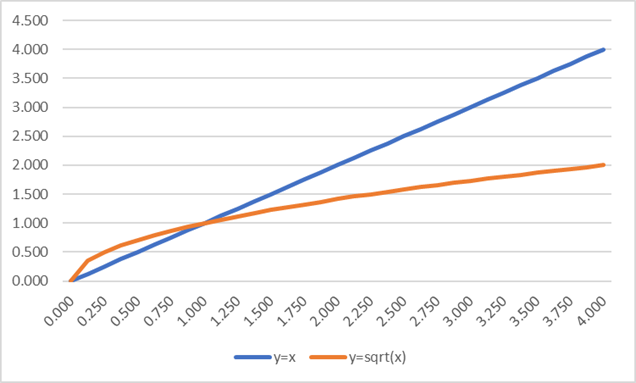
Quindi l’impatto è lineare rispetto al multiplo (q/ADV), cioè i giorni necessari per smaltire un ordine, dipende dalla radice quadrata dell’orizzonte in modo inverso, in accordo con il modello di evoluzione del prezzo pilotato dal moto browniano, infine da un parametro c da calibrare, indicato in vari studi tra 0.3 e 0.5

4 Stato dell’arte normativo. Azioni di controllo delle autorità

A seguito della entrata in vigore delle linee guida ESMA alla fine del 2020, sono state condotte delle attività di controllo sulla qualità delle implementazioni da parte dei gestori dei fondi comuni.

 In particola ESMA ha lanciato nel 2020 la common survey Action (CSA) sul tema del liquidity risk presso i gestori dei fondi sottoponendo un modulo molto dettagliato per la raccolta di dati relativi a processi, alle policy, alle metodologie e ai sistemi di controllo del liquidity risk.

A questa raccolta è seguita una comunicazione nel marzo 2021 con le principali risultanze, si veda [4]. Comunicazione ripresa poi da Banca d’Italia verso tutti i gestori sotto la sua supervisione con analoga iniziativa, in data 25.5.2021.

In tali report si esprimono una serie di punti di debolezza degli apparati di controllo del liquidity risk, che seguendo la comunicazione Banca d’Italia possiamo strutturare nei seguenti aspetti:

  1. Mancanza o fragilità dei sistemi di pre-deal check, per il controllo ex-ante dei profili di liquidità delle nuove operazioni, con eccesso di fiducia sulla liquidità degli strumenti quotati
  2. Metodi di misura nel continuo da migliorare, con richiesta di rendere più importanti le misure di tipo TTL (time to liquidate), di tenere conto del fabbisogno di liquidità per le margin call di operazioni in derivati, e di formulare scenari sul passivo più articolati
  3. Eccessiva passività rispetto a dati e modelli dei provider esterni, con richiesta di avere capacità proprie di data quality e benchmarking
  4. Miglioramento dei processi, con formalizzazione di limiti, ruoli, azioni di remediation.

È stato chiesto a tutte le SGR di rispondere su tali punti di debolezza entro il 31.10.2021 e poi sono stati avviate dove necessarie interazioni dirette tra le autohorities e la singola società di gestione.

Qualche commento su questi punti di debolezza. Se da un lato sono tutti condivisibili da una prospettiva generale, alcuni di questi presentano obiettive difficoltà pratiche.

Per esempio, un controllo ex-ante sugli impatti di liquidità sconta molte assunzioni, necessità di molti dati, scenari assolutamente molto incerti, difficoltà tecnica di reale integrazione nei sistemi di position keeping di inserimento degli ordini.

Oppure, la richiesta di avere modelli indipendenti di calcolo, per SGR piccole che possono comunque avere un universo investito di migliaia di diversi strumenti, viola il principio di proporzionalità, e la sua asseverazione implicherebbe costi rilevanti rispetto al sistema di costi e ricavi di realtà medio piccole, sia in termini di provider alternativi, sia di sviluppo modelli e relativi software proprietari.

Riferimenti

[1] Banca d’Italia (2015), “Regolamento sulla Gestione Collettiva del Risparmio“

[2] ESMA (2019), “Guidelines on liquidity stress testing in UCITS and AIF” ESMA GL 34-39-881

[3] ESMA (2019), “Stress simulation for investment funds “ESMA GL 50-164-2458

[4] ESMA (2021), “Results of the 2020 Common Supervisory Action (CSA) on UCITS liquidity risk management”

[5] Acerbi C. e Scandolo G. (2008), “Liquidity Risk Theory and Coherent Measures of Risk”

[6] Lillo F. et al (2014), “Beyond the square root: Evidence for logarithmic dependence of market impact on size and participation rate”

[7] Cont, R. and Schaanning, E. (2017), “Fire sales, indirect contagion and systemic stress testing”, Norges Bank Working Paper No. 2.

Ringraziamenti

Si ringraziano Dr. Bianca Garavaglia, AcomeA SGR, e Dr. Simone Frigerio, BCC Risparmio e Previdenza SGR, per le proficue interazioni sul tema.