

Stress test: un quadro non del tutto positivo ma più veritiero del passato
di Emilio Barucci e Carlo Milani

Nov 11 2018
Stress test: un quadro non del tutto positivo ma più veritiero del passato   di Emilio Barucci e Carlo Milani

Lo scorso 2 novembre l’EBA ha diffuso i risultati della nuova tornata di stress test condotta durante il 2018 a partire dai dati di bilancio relativi alla fine del 2017. Il test ha riguardato 48 banche operanti in 15 paesi europei ed ha fornito indicazioni sui coefficienti (attesi) di patrimonializzazione nello scenario base e in quello avverso per un orizzonte temporale che arriva al 2020. Per l’Italia sono state considerate 4 banche: Unicredit, Intesa-Sanpaolo, Ubi e Banco BPM.

Come per gli stress test condotti nel 2016 l’intento dell’EBA non è quello di decretare in modo esplicito gli istituti che falliscono il test quanto quello di utilizzare le informazioni per il Supervisory Review and Evaluation Process (SREP) al fine di definire i requisiti aggiuntivi di capitale richiesti alle singole banche per tener conto del loro grado di rischiosità.

L’assenza di una lista di “vincitori e vinti” ha permesso a molte banche di dichiararsi tra quelle che hanno superato meglio il test, un po’ sulla falsa riga di Donald Trump che ha sbandierato una vittoria al Senato nelle elezioni di midterm omettendo l’amissione della sconfitta alla Camera dei rappresentanti.

I dati presentati nel report dell’EBA si prestano infatti a diverse interpretazioni a seconda dell’indicatore di patrimonializzazione considerato e della grandezza osservata. Prendendo a riferimento il Common Equity Tier1 (CET1) ratio fully loaded (ovvero il ratio che incorpora gli effetti a regime della piena implementazione della Capital Requirements Regulation, della Capital Requirements Directive IV e del principio contabile IFRS 9) e il leverage ratio, sempre fully loaded, si ha una diversa fotografia. Il primo indicatore (CET1 raio) è influenzato dal modello di business della banca, dal livello di rischio degli assets e dall’utilizzo dei modelli interni per la valutazione del rischio. Il secondo indicatore (leverage ratio), avendo al denominatore una grandezza non ponderata per il rischio, ha il pregio di non risentire degli effetti della potenziale manipolazione delle attività ponderate per il rischio (Barucci e Milani, 2018).


Grafico 1. Effetto dello scenario di stress al 2020

Fonte: elaborazioni BEM Research su dati EBA.


Nel grafico 1 è riportato l’effetto al 2020 sui due coefficienti di patrimonializzazione dello scenario di stress in termini di basis points. Le 48 banche considerate sono state aggregate in base al paese di origine. Dal grafico emerge che sulla base del CET1 ratio il Regno Unito e la Germania sono i due sistemi che subirebbero i maggiori contraccolpi nello scenario avverso. In media le banche inglesi vedrebbero ridursi il loro CET1 ratio di oltre 600 punti base (bp), quelle tedesche di circa 560. Pesante sarebbe anche l’effetto sulle banche irlandesi, finlandesi e danesi (circa 500 bp). Le banche italiane, invece, avrebbero un impatto di circa 350 bp, che si colloca leggermente al di sotto della media complessiva (370 bp).

Sulla base di queste evidenze alcuni giornali italiani hanno titolato sottolineando il fatto che le banche italiane siano tra le “vincitrici” dell’ultima tornata di stress test. Questa interpretazione racconta solo una parte della storia. Basta guardare al dato circa l’impatto dello scenario avverso sul leverage ratio per trovare una fotografia in parte diversa. Sulla base di questo indicatore sono le banche irlandesi quelle più colpite (200 bp), seguite dalle finlandesi (150 bp), dalle austriache (140 bp) e dalle inglesi (130 bp). In questo caso le banche italiane, con un impatto negativo medio di 115 bp, si posizionano al di sopra della media europea (90 bp), ad un livello non molto distante da quanto osservato per gli istituti tedeschi. Ci possiamo rasserenare per il fatto che il primo pilastro della regolamentazione si basa pur sempre sul CET ratio ma il dato non può essere trascurato.

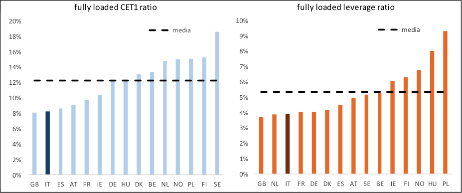
Ancor meno rassicurante è il dato che emerge osservando il livello medio di CET1 ratio e di leverage ratio ottenuti negli scenari di stress (grafico 2). In questo caso le banche italiane sono in media tra quelle che evidenziano, per entrambi gli indicatori, coefficienti tra i più bassi in Europa.


Grafico 2. Coefficienti di patrimonializzazione al 2020 nello scenario stressato
Fonte: elaborazioni BEM Research su dati EBA.


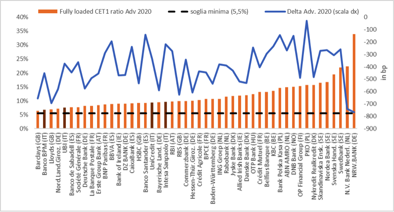
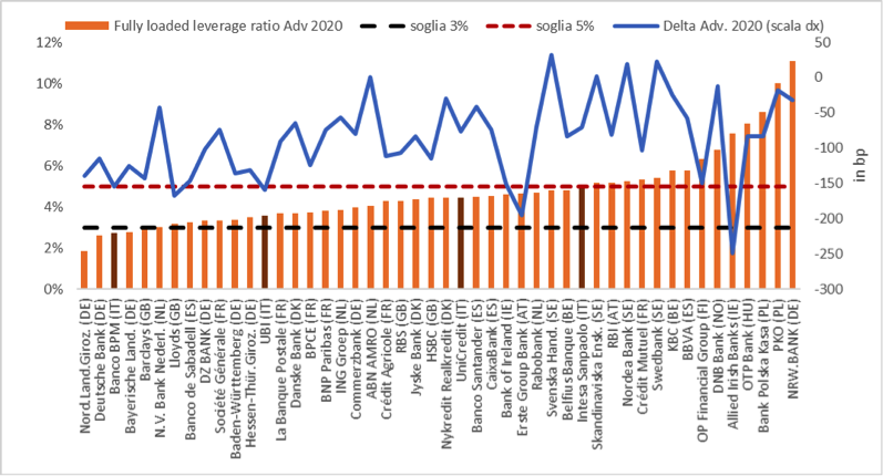
Guardando al dettaglio per singola banca si rileva che sono in particolare Banco BPM e UBI ad evidenziare livelli contenuti sia sul CET1 ratio sia sul leverage ratio (grafici 3 e 4).

Leggendo assieme il grafico 1 e il grafico 2 possiamo dedurre che le banche italiane sono sì meno esposte delle altre europee ai rischi macroeconomici ma sono ancora sottocapitalizzate: quindi una variazione non elevata in termini di capital ratio le porta ad un basso coefficiente di patrimonializzazione. A ben guardare è la Gran Bretagna ad essere messa male sotto ambedue i profili.

Da notare in particolare come il leverage ratio, nello scenario stressato, scenderebbe al di sotto della soglia del 3%, prevista da Basilea 3, in diverse realtà bancarie europee, tra cui anche Deutsche Bank e Banco BPM. Solo 21 tra le 48 banche considerate avrebbero invece nel 2020 un leverage ratio post stress test al di sopra del 5%, la soglia imposta dalla Federal Reserve e dal Federal Deposit Insurance Corporation (FDIC) alle banche operanti negli Stati Uniti.


Grafico 3. Fully loaded CET1 ratio al 2020 nello scenario stressato e scarti rispetto alla baseline
Fonte: elaborazioni BEM Research su dati EBA.

Grafico 4. Fully loaded leverage ratio al 2020 nello scenario stressato e scarti rispetto alla baseline
Fonte: elaborazioni BEM Research su dati EBA.

In definitiva, i risultati degli stress test per il 2018 non sembrano essere così rassicuranti come qualche commentatore ha evidenziato. Oltretutto occorre rilevare che, come spesso è accaduto in passato le ipotesi adottate dall’EBA per disegnare gli scenari degli stress sono state superate dalla realtà in due direzioni. Al riguardo occorre notare che per l’Italia lo scenario avverso ha ipotizzato un calo consistente del Pil (7 punti percentuali cumulati fino al 2020) ma con uno spread BTP-Bund pari a 250 bp (Milani, 2018), quando invece nel periodo recente ha toccato quota 340 bp oscillando su valori intorno ai 300 bp.

Le notizie ‘‘positive’’ vengono soprattutto dal fatto che la performance ‘‘negativa’’ in termini di variazione del capital ratio delle banche inglesi, tedesche e dei paesi nordici è dovuta al fatto che finalmente gli stress tests sono in grado di ‘‘stressare’’ gli asset di livello II e III, che sono presenti soprattutto nelle banche dei paesi del nord Europa. Si tratta di titoli complessi, difficili da valutare che sono state all’origine della crisi finanziaria ed erano stati ignorati dall’EBA nelle analisi precedenti, si veda al riguardo Barucci, Baviera e Milani (2018). D’altro canto, la pulizia dei bilanci delle banche italiane dei NPL ha sicuramente avuto un effetto positivo nel renderle meno rischiose.

Bibliografia

  • Barucci E., R. Baviera, C. Milani, The Comprehensive Assessment: What lessons can be learned?,  The European Journal of Finance, 2018.
  • Barucci E., C. Milani, Do European banks manipulate risk weights?, International Review of Financial Analysis, Volume 59, pp. 47-57, North-Holland, 2018.
  • Milani C., Le principali caratteristiche degli stress test 2018, finriskalert.it del 12 febbraio 2018.

BIS: distributed ledger technology and large value payments

Nov 10 2018

Mr Hyun Song Shin, Economic Adviser and Head of Research of the Bank for International Settlement (BIS), examines the liquidity properties of decentralised payment systems in an economic model of payments, in which the cost of credit to finance payments enters explicitly.

Payment systems built around distributed ledger technology (DLT) operate by maintaining identical copies of the history of payments among the participant nodes in the payment system. Cryptocurrencies are perhaps the best-known example of the application of DLT, but the applicability of the technology is much broader. Payment systems based on DLT are compatible with oversight by the central bank, and several central banks have conducted successful trials of interbank payments. In these trials, payment system participants transfer digital tokens that are redeemable at the central bank and use DLT to transfer them to other system participants. Decentralised consensus is achieved through agreement of a supermajority of the participants (typically 75-80%) who collectively validate payments.

Nevertheless, the technology by itself does not overcome the credit needs of the payment system to maintain settlement liquidity. In conventional real-time gross settlement (RTGS) payment systems, the value of daily payments can be over 100 times the deposit balance maintained by the system participant at the central bank. As such, incoming payments are recycled into outgoing payments, and credit provided by the central bank supplements private credit from outside the payment system for the smooth functioning of the system as a whole.

In a two-bank example, we illustrate the conceptual distinction between consensus as distributed knowledge and consensus strong enough to sustain a cooperative outcome. In this example, when the cost of credit exceeds a modest threshold, no amount of exchange of messages can elicit the coordination of payments between the two banks. The example focuses attention on the coordination motives of system participants. The cost of credit turns out to be a key determinant of the equilibrium outcome of the game.

We then proceed to examine a general N-bank game and cast the payment problem as a public good contribution game between N banks in a large-value payment system. The public good has two aspects. The first aspect of the public good is the availability of a clean, reconciled ledger that commands agreement from system participants. This part is where the technological innovation can contribute most.

The second aspect of the public good is the provision of credit to clients which allows high volume of outgoing payments that sustains the coordination outcome with high flows. We solve for the unique, dominance-solvable equilibrium using global game techniques and provide an exact characterisation of the states of the world at which the coordination outcome is feasible.

The solution shows that successful coordination is possible in a decentralised setting, but only within a narrow range of fundamentals. The solution is highly sensitive to the cost of credit, and the decentralised equilibrium outcome often fails to reproduce the high-volume payment outcomes that are more normal with central bank balance sheet backing.

Payment systems built around distributed ledger technology (DLT) operate by maintaining identical copies of the history of payments among the participant nodes in the payment system. Cryptocurrencies are perhaps the best-known example of the application of DLT, but the applicability of the technology is much broader. Payment systems based on DLT are compatible with oversight by the central bank, and several central banks have conducted successful trials of interbank payments. In these trials, payment system participants transfer digital tokens that are redeemable at the central bank and use DLT to transfer them to other system participants. Decentralised consensus is achieved through agreement of a supermajority of the participants (typically 75-80%) who collectively validate payments.

Nevertheless, the technology by itself does not overcome the credit needs of the payment system to maintain settlement liquidity. In conventional real-time gross settlement (RTGS) payment systems, the value of daily payments can be over 100 times the deposit balance maintained by the system participant at the central bank. As such, incoming payments are recycled into outgoing payments, and credit provided by the central bank supplements private credit from outside the payment system for the smooth functioning of the system as a whole.

Distributed ledger technology and large value payments: a global game approach (PDF)

ESMA warns CRAs and TRs to prepare for a no-deal Brexit

Nov 10 2018

The European Securities and Markets Authority (ESMA) issued a Public Statement in order to raise market participants’ awareness on the readiness of credit rating agencies (CRAs) and trade repositories (TRs) for the possibility of no agreement being reached in the context of the United Kingdom (UK) withdrawing from the European Union (EU).

As there is no assurance that a transition period will be agreed, entities using services provided by CRAs and TRs need to consider the scenario where a no-deal Brexit would take place on 30 March 2019.

Derivatives subject to the reporting obligation under EMIR1 must be reported to a registered EU-established TR or a recognised third-country TR2. Similarly, CRAs need to have a legal entity registered in the EU and supervised by ESMA, in order for their ratings to be used for regulatory purposes in the EU. In a no-deal Brexit scenario, TRs and CRAs established in the UK will lose their EU registration as of the UK’s withdrawal date.

UK-based CRAs and TRs currently registered with ESMA have implemented contingency plans in preparation of a no-deal Brexit scenario. ESMA has noted significant steps forward by both industry sectors in terms of preparedness, however, some actions still need to be completed.

ESMA is engaging on a continuous basis with the relevant supervised entities to ensure that the agreed Brexit contingency plans are fully executed by March 2019 in case of no- deal Brexit, including the finalisation of pending applications for registration. ESMA is currently assessing a number of CRAs and TRs applications, submitted as part of the firms’ Brexit contingency plans.

ESMA emphasises that a positive decision on a registration application ultimately depends on the completeness and the quality of the application file and on the applicant’s compliance with the relevant regulations.

EU counterparties and CCPs must report details of derivative contracts to a registered EU- established TR or a recognised third-country TR. All counterparties must ensure that this requirement continues to be fulfilled. ESMA invites market participants to contact their TR to verify whether continuity of service will be ensured after Brexit.

In general, ESMA emphasises the importance for market participants to monitor closely the public disclosures made by CRAs and TRs in the context of Brexit.


ESMA: Contingency plans of Credit Rating Agencies and Trade Repositories in the context of the United Kingdom withdrawing from the European Union (PDF)


FSB: SME financing, the use of SupTech and RegTech, and implementation of the Net Stable Funding Ratio

Nov 10 2018

The Financial Stability Board (FSB) Regional Consultative Group (RCG) for the Middle East and North Africa (MENA) met in Istanbul today at a meeting hosted by the Central Bank of the Republic of Turkey.

Members of the FSB RCG MENA received an update on the FSB’s work programme and deliverables for the G20 Leaders’ Summit later this month in Buenos Aires, including evaluations of the effects of the reforms on infrastructure finance and on incentives to centrally clear over-the-counter derivatives, and a progress report on the FSB action plan to assess and address the decline in correspondent banking relationships. The FSB’s work in 2019 and beyond will focus on (i) finalising and operationalising post-crisis reforms; (ii) monitoring the implementation and evaluating the effects of post-crisis reforms; and (iii) addressing new and emerging vulnerabilities in the financial system.

Turning to vulnerabilities and regional financial stability issues, meeting participants noted that, while global growth remains strong, the recovery is less balanced and financial conditions could tighten, particularly in emerging markets. For the MENA region specifically, members expect economic growth in oil exporting countries to rebound, while importing countries may remain challenged. The region’s banking sector remains generally sound with improved liquidity positions, but non-performing loan levels are high in some countries. Credit growth is modest and could be further impacted by rising interest rates.

Members next considered financing to small and medium-sized enterprises (SMEs) and their role in the region’s economic development. Although SMEs traditionally present more credit risk than large corporates, the level of risk in SMEs has declined in recent years, while credit and business conditions have improved. These positive developments, however, have not always translated into greater access to financing. Members discussed both financial and non-financial impediments to SME lending in the region. The FSB is conducting an evaluation of the effects of the G20 financial regulatory reforms on SME financing, and will publish a consultative paper by mid-2019 and a final report by end-2019.

The group discussed how technology can be leveraged to achieve supervisory and regulatory objectives (SupTech). They considered the potential uses of SupTech and how to facilitate innovation while at the same time maintaining effective oversight. They also exchanged views on how it could change supervision in the future and some of the challenges that technology might raise for financial sector supervisors, such as the skill sets that they will need, oversight of decentralised systems and distributed ledgers, and data protection. Members also discussed the use of technology such as big data and machine learning to help financial institutions comply with regulatory requirements (RegTech).

Finally, members discussed implementation of the Basel Committee’s net stable funding ratio (NSFR) and its effects on banks in the region. They reviewed the objectives and key elements of the NSFR, as well as implementation challenges such as those faced by banks when attempting to adjust their information systems to meet and report on the new requirements. Several jurisdictions in the region have either issued final rules for the implementation of the NSFR or are in the process of doing so.


FSB: RCG on MENA NOV 18 – Full text (PDF)

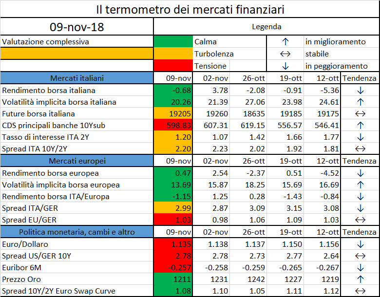
Il termometro dei mercati finanziari (9 novembre 2018)
a cura di Emilio Barucci e Daniele Marazzina

Nov 10 2018
Il termometro dei mercati finanziari (9 novembre 2018)  a cura di Emilio Barucci e Daniele Marazzina

L’iniziativa di Finriskalert.it “Il termometro dei mercati finanziari” vuole presentare un indicatore settimanale sul grado di turbolenza/tensione dei mercati finanziari, con particolare attenzione all’Italia.

Significato degli indicatori

  • Rendimento borsa italiana: rendimento settimanale dell’indice della borsa italiana FTSEMIB;
  • Volatilità implicita borsa italiana: volatilità implicita calcolata considerando le opzioni at-the-money sul FTSEMIB a 3 mesi;
  • Future borsa italiana: valore del future sul FTSEMIB;
  • CDS principali banche 10Ysub: CDS medio delle obbligazioni subordinate a 10 anni delle principali banche italiane (Unicredit, Intesa San Paolo, MPS, Banco BPM);
  • Tasso di interesse ITA 2Y: tasso di interesse costruito sulla curva dei BTP con scadenza a due anni;
  • Spread ITA 10Y/2Y : differenza del tasso di interesse dei BTP a 10 anni e a 2 anni;
  • Rendimento borsa europea: rendimento settimanale dell’indice delle borse europee Eurostoxx;
  • Volatilità implicita borsa europea: volatilità implicita calcolata sulle opzioni at-the-money sull’indice Eurostoxx a scadenza 3 mesi;
  • Rendimento borsa ITA/Europa: differenza tra il rendimento settimanale della borsa italiana e quello delle borse europee, calcolato sugli indici FTSEMIB e Eurostoxx;
  • Spread ITA/GER: differenza tra i tassi di interesse italiani e tedeschi a 10 anni;
  • Spread EU/GER: differenza media tra i tassi di interesse dei principali paesi europei (Francia, Belgio, Spagna, Italia, Olanda) e quelli tedeschi a 10 anni;
  • Euro/dollaro: tasso di cambio euro/dollaro;
  • Spread US/GER 10Y: spread tra i tassi di interesse degli Stati Uniti e quelli tedeschi con scadenza 10 anni;
  • Prezzo Oro: quotazione dell’oro (in USD)
  • Spread 10Y/2Y Euro Swap Curve: differenza del tasso della curva EURO ZONE IRS 3M a 10Y e 2Y;
  • Euribor 6M: tasso euribor a 6 mesi.

I colori sono assegnati in un’ottica VaR: se il valore riportato è superiore (inferiore) al quantile al 15%, il colore utilizzato è l’arancione. Se il valore riportato è superiore (inferiore) al quantile al 5% il colore utilizzato è il rosso. La banda (verso l’alto o verso il basso) viene selezionata, a seconda dell’indicatore, nella direzione dell’instabilità del mercato. I quantili vengono ricostruiti prendendo la serie storica di un anno di osservazioni: ad esempio, un valore in una casella rossa significa che appartiene al 5% dei valori meno positivi riscontrati nell’ultimo anno. Per le prime tre voci della sezione “Politica Monetaria”, le bande per definire il colore sono simmetriche (valori in positivo e in negativo). I dati riportati provengono dal database Thomson Reuters. Infine, la tendenza mostra la dinamica in atto e viene rappresentata dalle frecce: ↑,↓, ↔  indicano rispettivamente miglioramento, peggioramento, stabilità.

Disclaimer: Le informazioni contenute in questa pagina sono esclusivamente a scopo informativo e per uso personale. Le informazioni possono essere modificate da finriskalert.it in qualsiasi momento e senza preavviso. Finriskalert.it non può fornire alcuna garanzia in merito all’affidabilità, completezza, esattezza ed attualità dei dati riportati e, pertanto, non assume alcuna responsabilità per qualsiasi danno legato all’uso, proprio o improprio delle informazioni contenute in questa pagina. I contenuti presenti in questa pagina non devono in alcun modo essere intesi come consigli finanziari, economici, giuridici, fiscali o di altra natura e nessuna decisione d’investimento o qualsiasi altra decisione deve essere presa unicamente sulla base di questi dati.

ECB: Monetary policy and climate change

Nov 10 2018

Benoît Cœuré, Member of the Executive Board of the ECB spoke of the connection between monetary policy and climate changes at the conference on “Scaling up Green Finance: The Role of Central Banks”, organised by the Network for Greening the Financial System, the Deutsche Bundesbank and the Council on Economic Policies on the 8 November 2018.

He started observing that, without further mitigation, cumulative emissions pose significant risks of economic disruption. There is a wide recognition that environmental externalities should be primarily corrected by first-best policies, such as taxes, hence all authorities, including the ECB, need to consider the appropriate response to climate change.

The Financial Stability Board’s Task Force on Climate-related Financial Disclosures published its first status report just a few weeks ago. Only last week, ECB Banking Supervision communicated to banks that climate-related risks have been identified as being among the key risk drivers affecting the euro area banking system.

Yet an area that has received less attention though, both in policy and in academia, is the impact of climate change on the conduct of monetary policy. He argues that climate change can further complicate the correct identification of shocks relevant for the medium-term inflation outlook, it may increase the likelihood of extreme events and hence erode central banks’ conventional policy space more often, and it may raise the number of occasions on which central banks face a trade-off forcing them to prioritise stable prices over output.

To appreciate how climate change may affect monetary policy, it is useful to first recall the basic principles of how central banks decide on their actions. Broadly speaking, implementing monetary policy is the practice of identifying the nature, persistence and magnitude of the shocks hitting the economy. Policymakers typically differentiate between two broad categories of shocks.

The first is demand shocks. These are shocks that are “benign” or manageable from the perspective of monetary policy because they pull inflation, growth and employment in the same direction – a “divine coincidence” which does not pose a dilemma to central banks. The second category relates to supply-side shocks. These shocks are less easy to accommodate for central banks as they pull output and inflation in opposite directions. This generates a trade-off for central banks between stabilising inflation and stabilising output fluctuations. Climate-related shocks typically fall into this second category of shocks.

Droughts and heatwaves often lead to crop shortfalls, putting upward pressure on food prices.Hurricanes and floods destroy production capacity, thereby raising input and output prices. And unusually cold winters can be seen as malign productivity shocks – that is, they may raise input prices for the same level of output.

So, much like other supply shocks, weather-related disturbances typically pose a dilemma for central banks, which may then have to choose between stabilising inflation or economic activity. Policymakers have usually resolved this trade-off by calibrating their response to a supply-side shock according to its estimated persistence and size.

If the shock is thought to be short-lived, and unlikely to affect the medium-term inflation outlook relevant for monetary policy, we usually “look through” the shock – that is, we tolerate its temporary effects on inflation without taking any action. If the effects prove more persistent, however, and are at risk of spreading more widely through the economy, monetary policy action may be warranted.

It is fair to say that most weather-related shocks have been short-lived and contained – at least so far. This year’s extremely hot and dry summer, for example, meant smaller harvests for many European farmers. But its overall price effects have been limited to vegetable prices, and will probably prove to be temporary. Similarly, although the flooding in June 2013 was the most severe in Germany since the 1950s, its macroeconomic impact was limited. As a result, the ECB, in its short history, has never yet been compelled to take action in response to climate-related shocks. So far their largely temporary effects on output and inflation have allowed us to look through them. This meant that central bankers thought the horizon of climate change was extending well beyond the one of monetary policy.

But this may change – he argues – the horizon at which climate change impacts the economy has shortened, warranting a discussion on how it affects the conduct of monetary policy. That is, climate change is likely to affect monetary policy one way or the other – whether it is left unchecked or humankind rises to the climate change challenge.

In recent years, for example, we have repeatedly observed an unusual blip in economic activity in the United States in the first quarter. This has often been attributed to a harsh winter, despite best efforts to seasonally adjust the data. But causality is inherently difficult to establish. Indeed, statistical analysis has challenged the hypothesis that cold temperatures are behind the observed deceleration in first-quarter growth.

Similarly, last month, we saw a puzzling persistence in petroleum prices in Germany despite a parallel fall in oil prices. One hypothesis is that this year’s hot summer caused the water levels in German rivers to fall to levels that only allow petrol tankers to carry half their capacity, creating supply bottlenecks.

It will thus become increasingly difficult for central banks to disentangle the variation in the data relevant for the assessment of the medium-term inflation outlook. It will cause the signal-to-noise ratio to deteriorate and thereby increase the risk that central banks take action when in fact they shouldn’t, or vice versa.

Furthermore, the longer the risks of climate change are ignored, the higher the risks of catastrophic events, possibly with irreversible consequences for the economy. In other words, the distribution of shocks may become more “fat-tailed”.

The concern is that monetary policy may be more often forced to adopt non-standard policy measures. The global financial crisis has shown that extreme events can quickly erode central banks’ conventional policy space. Catastrophic climate change could thus test the limits of how far monetary policy can go and, in the extreme, force us to rethink our current policy framework.

The third and final implication relates to the persistence of shocks and the inflation-output trade-off central banks may face. Climate change, for example, will make some areas of the world less habitable, which can be expected to increase the frequency and intensity of international migration. The events of recent years, though different in nature, highlight how migration can have long-lasting effects on broader labour market dynamics and, ultimately, wage developments. There is evidence that migration has contributed to dampening wage growth in Germany in recent years, thereby further complicating our efforts to bring inflation back to levels closer to 2%.

Similarly, in the absence of clear and tangible evidence that the demand for fossil fuels will decline, and with existing conventional oil fields depleting rapidly, persistent energy shocks cannot be ruled out.

More frequent climate-related shocks may increasingly blur the analysis of the medium-term inflationary pressures relevant for monetary policy. More fat-tailed shocks may erode central banks’ conventional policy space more often in the future. The ECB will thus concentrate its efforts on supporting market participants, legislators and standard-setting bodies in identifying the risks emerging from climate change and providing a clear framework to reorient financial flows and reduce such risks. A unified framework is the gravitational force needed to finance the greening of our economy.

Monetary policy and climate change: complete speech (HTML)

Il termometro dei mercati finanziari (2 novembre 2018)
a cura di Emilio Barucci e Daniele Marazzina

Nov 03 2018
Il termometro dei mercati finanziari (2 novembre 2018)  a cura di Emilio Barucci e Daniele Marazzina

L’iniziativa di Finriskalert.it “Il termometro dei mercati finanziari” vuole presentare un indicatore settimanale sul grado di turbolenza/tensione dei mercati finanziari, con particolare attenzione all’Italia.

Significato degli indicatori

  • Rendimento borsa italiana: rendimento settimanale dell’indice della borsa italiana FTSEMIB;
  • Volatilità implicita borsa italiana: volatilità implicita calcolata considerando le opzioni at-the-money sul FTSEMIB a 3 mesi;
  • Future borsa italiana: valore del future sul FTSEMIB;
  • CDS principali banche 10Ysub: CDS medio delle obbligazioni subordinate a 10 anni delle principali banche italiane (Unicredit, Intesa San Paolo, MPS, Banco BPM);
  • Tasso di interesse ITA 2Y: tasso di interesse costruito sulla curva dei BTP con scadenza a due anni;
  • Spread ITA 10Y/2Y : differenza del tasso di interesse dei BTP a 10 anni e a 2 anni;
  • Rendimento borsa europea: rendimento settimanale dell’indice delle borse europee Eurostoxx;
  • Volatilità implicita borsa europea: volatilità implicita calcolata sulle opzioni at-the-money sull’indice Eurostoxx a scadenza 3 mesi;
  • Rendimento borsa ITA/Europa: differenza tra il rendimento settimanale della borsa italiana e quello delle borse europee, calcolato sugli indici FTSEMIB e Eurostoxx;
  • Spread ITA/GER: differenza tra i tassi di interesse italiani e tedeschi a 10 anni;
  • Spread EU/GER: differenza media tra i tassi di interesse dei principali paesi europei (Francia, Belgio, Spagna, Italia, Olanda) e quelli tedeschi a 10 anni;
  • Euro/dollaro: tasso di cambio euro/dollaro;
  • Spread US/GER 10Y: spread tra i tassi di interesse degli Stati Uniti e quelli tedeschi con scadenza 10 anni;
  • Prezzo Oro: quotazione dell’oro (in USD)
  • Spread 10Y/2Y Euro Swap Curve: differenza del tasso della curva EURO ZONE IRS 3M a 10Y e 2Y;
  • Euribor 6M: tasso euribor a 6 mesi.

I colori sono assegnati in un’ottica VaR: se il valore riportato è superiore (inferiore) al quantile al 15%, il colore utilizzato è l’arancione. Se il valore riportato è superiore (inferiore) al quantile al 5% il colore utilizzato è il rosso. La banda (verso l’alto o verso il basso) viene selezionata, a seconda dell’indicatore, nella direzione dell’instabilità del mercato. I quantili vengono ricostruiti prendendo la serie storica di un anno di osservazioni: ad esempio, un valore in una casella rossa significa che appartiene al 5% dei valori meno positivi riscontrati nell’ultimo anno. Per le prime tre voci della sezione “Politica Monetaria”, le bande per definire il colore sono simmetriche (valori in positivo e in negativo). I dati riportati provengono dal database Thomson Reuters. Infine, la tendenza mostra la dinamica in atto e viene rappresentata dalle frecce: ↑,↓, ↔  indicano rispettivamente miglioramento, peggioramento, stabilità.

Disclaimer: Le informazioni contenute in questa pagina sono esclusivamente a scopo informativo e per uso personale. Le informazioni possono essere modificate da finriskalert.it in qualsiasi momento e senza preavviso. Finriskalert.it non può fornire alcuna garanzia in merito all’affidabilità, completezza, esattezza ed attualità dei dati riportati e, pertanto, non assume alcuna responsabilità per qualsiasi danno legato all’uso, proprio o improprio delle informazioni contenute in questa pagina. I contenuti presenti in questa pagina non devono in alcun modo essere intesi come consigli finanziari, economici, giuridici, fiscali o di altra natura e nessuna decisione d’investimento o qualsiasi altra decisione deve essere presa unicamente sulla base di questi dati.

Basel committee: progress report on adoption of the Basel regulatory framework

Nov 02 2018

The Basel Committee is publishing the fifteenth progress report on adoption of the Basel regulatory framework, October 2018. The report sets out the adoption status of Basel III standards for each Basel Committee on Banking Supervision (BCBS) member jurisdiction as of end-September 2018.

In 2012, the Committee started the Regulatory Consistency Assessment Programme (RCAP) to monitor progress in introducing domestic regulations, assessing their consistency and analysing regulatory outcomes. As part of this programme, the Committee periodically monitors the adoption of Basel standards. The monitoring initially focused on the Basel risk-based capital requirements, and has since expanded to cover all Basel standards. These include the finalised Basel III post-crisis reforms published by the Committee in December 2017, which will take effect from 1 January 2022 and will be phased in over five years. When those reforms were published, the Group of Central Bank Governors and Heads of Supervision, the oversight body of the BCBS, reaffirmed its expectation of full, timely and consistent implementation of all elements of the package.

As of end-September 2018, all 27 member jurisdictions have risk-based capital rules, liquidity coverage ratio (LCR) regulations and capital conservation buffers in force. Twenty-six member jurisdictions also have final rules in force for the countercyclical capital buffer and the domestic systemically important bank (D-SIB) requirement. With regard to the global systemically important bank (G-SIB) requirements published in 2013, all members that are home jurisdictions to G-SIBs have final rules in force.

Since the last report published in April 2018, member jurisdictions have made further progress in implementing standards whose deadline has already passed. These include the leverage ratio based on the existing (2014) exposure definition, which is now partly or fully implemented in 26 member jurisdictions. Moreover, 25 member jurisdictions have issued draft or final rules for the Net Stable Funding Ratio (NSFR), and 20 member jurisdictions have issued draft or final rules for the revised securitisation framework.

In case of implementation of the standardised approach for measuring counterparty credit risk exposures (SA-CCR), 24 member jurisdictions have issued draft or final rules. Also, draft or final rules for the capital requirements for bank exposures to central counterparties (CCPs) have been issued by 23 member jurisdictions. However, in many jurisdictions, rules for these standards are yet to be finalised and come into force. This is notably the case for the NSFR, with only 10 member jurisdictions having final rules in force as of end-September 2018.

There has been also progress in implementation of standards whose deadline is within the next six months. On requirements for total loss-absorbing capacity (TLAC), 15 member jurisdictions have issued draft or final rules. Similarly, 21 member jurisdictions have issued draft or final rules for the large exposure (LEX) framework and for interest rate risk in the banking book (IRRBB).

Draft or final rules published and reported by member jurisdictions between end-September 2018 and the publication of this report may be taken into account. However, limited progress has been observed in the implementation of capital requirements for equity investments in funds.

While the Committee welcomes the progress made on the implementation of various standards by member jurisdictions, it urges them to strive for full, timely and consistent implementation of Basel III post-crisis reforms and will continue monitoring closely the implementation of these reforms.

Regarding the consistency of regulatory implementation, the Committee has published its assessment reports on all 27 members regarding their implementation of Basel risk-based capital and LCR standards. Further, assessments of implementation of the Basel G-SIB framework were published in June 2016, covering the five jurisdictions that are currently home to G-SIBs.

In 2018, the Committee has started assessing the consistency of implementation of the NSFR and the LEX framework.5 The first such assessment was of the Kingdom of Saudi Arabia. Overall, the NSFR regulations and the LEX framework in Saudi Arabia were found to be “compliant” with the Basel standards.6 The Committee plans to complete its review of the implementation of the NSFR and the LEX framework for all member jurisdictions by September 2020.7

Regarding the analysis of consistency of regulatory outcomes, the Committee has published five reports on the regulatory consistency of risk-weighted assets in the banking book and in the trading book

Basel Committee: Fifteenth progress report on adoption of the Basel regulatory framework (PDF)

EBA: Guidelines on management of non-performing and forborne exposures

Nov 02 2018

The European Banking Authority (EBA) publishes today its final “Guidelines on management of non-performing and forborne exposures”. The Guidelines, developed in accordance with the European Council Action Plan, aim to ensure that credit institutions have adequate prudential tools and frameworks in place to manage effectively their non-performing exposures (NPEs) and to achieve a sustainable reduction on their balance sheets. To this end, the Guidelines require institutions to establish NPE reduction strategies and introduce governance and operational requirements to support them.

The Guidelines specify sound risk management practices for credit institutions in their management of NPEs and forborne exposures (FBEs), including requirements on NPE reduction strategies, governance and operations of NPE workout framework, internal control framework and monitoring. The Guidelines are written from a prudential perspective, but are also mindful of the pressing needs related to consumer protection to ensure that consumers are treated fairly.

The Guidelines also set out requirements for processes to recognise NPEs and FBEs, as well as a forbearance granting process with a focus on the viability of forbearance measures. In particular, the Guidelines specify that institutions should grant forbearance measures only with the view to return the borrower to a sustainable performing repayment status and are thus in the borrower’s interest.

The Guidelines introduce a threshold of 5% of gross NPL ratio as a trigger for developing NPE strategies and applying associated governance and operational arrangements. This threshold does not indicate an optimal level for NPLs and should not be considered as an automatic target to be used in credit institutions’ NPE strategies but sets a prudential framework for stricter supervisory monitoring to guard against rising levels of NPEs.

Finally, the Guidelines outline requirements for competent authorities’ assessment of credit institutions’ NPE management activity as part of the Supervisory Review and Evaluation Process (SREP).

The Guidelines, which are addressed to credit institutions and supervisors, take into account the proportionality aspects in their implementation and, where applicable, provide concrete examples in relation to small and less complex institutions.

Final Guidelines on management of non-performing and forborne exposures (PDF)

ESMA: new bond liquidity data available for MiFID II

Nov 02 2018

The European Securities and Markets Authority (ESMA) has today made available new data for bonds subject to the pre- and post-trade requirements of the Markets in Financial Instruments Directive (MiFID II) and Regulation (MiFIR) through its data register.

ESMA will start today to make available the third quarterly liquidity assessment for bonds available for trading on EU trading venues at the end of October. For this period, there are currently 470 liquid bonds subject to MiFID II transparency requirements.

ESMA’s liquidity assessment for bonds is based on a quarterly assessment of quantitative liquidity criteria, which include the daily average trading activity (trades and notional amount) and percentage of days traded per quarter. ESMA updates the bond market liquidity assessments quarterly. However, additional data and corrections submitted to ESMA may result in further updates within each quarter, published in FITRS (which shall be applicable the day following publication).

The full list of assessed bonds will be available through ESMA’s Financial Instruments Transparency System (FITRS) in the XML files with publication date from 31 October 2018 and through the Register web interface.In addition, as first communicated on 27 September 2018, ESMA is publishing for the first time the completeness indicators related to bond liquidity data.

ESMA: liquidity assessment (HTML)