Stablecoin issuer Tether reported $1.48 billion in net profit for the first quarter of the year, double the previous quarter’s result, according to its latest attestation published Wednesday….
Mag
10
2023
Stablecoin issuer Tether reported $1.48 billion in net profit for the first quarter of the year, double the previous quarter’s result, according to its latest attestation published Wednesday….

This article is about the risks faced by life insurance companies in a context of increasing rates. It starts with a brief recap of the Solvency II (SII) directive, and, after showing the recent development of the economic scenario, it reports how these risks are measured by the Standard Formula (SF), pointing out the solutions hinted by the market to overcome the drawbacks of the regulatory model, together with a description of a potential reinsurance treaty aimed at mitigating the impact on the capital requirements and position.
SII operates in a risk-based framework and requires insurers to hold sufficient capital to cover several quantifiable risks in very unfavorable situations. The capital adequacy is measured by the Solvency Ratio (SR), expressed as a ratio of Own Funds (OF – available capital, broadly Excess of Assets over Liabilities, EAoL) to Solvency Capital Requirement (SCR). According to the SF calculation, the SCR, to hold in addition to the Technical Provisions (TP), is obtained as the aggregation of modules of selected capital requirements, that cover the risks considered. Each capital requirement is calibrated as a Value at Risk (VaR) measure of the Basic OF (BOF), as impacted by that risk, based on their variation over one year, subject to a stress with a confidence level of 99.50%. As for the Assets, the TP are valued at a “fair price” and consist of a Best Estimate Liability (BEL) plus a Risk Margin (RM). The latter represents the theoretical compensation for the cost of holding regulatory capital against the risk that the future experience will be worse than the assumptions adopted for the BEL calculation. BEL values are defined as the present value of future expected Cash Flows (CFs), discounted by the means of a Risk-Free Rates (RFR) term structure, monthly published by EIOPA (European Insurance and Occupational Pension Authority), together with the prediction of its upward and downward stresses, used in the SCR Interest Rate (IR) risk module.
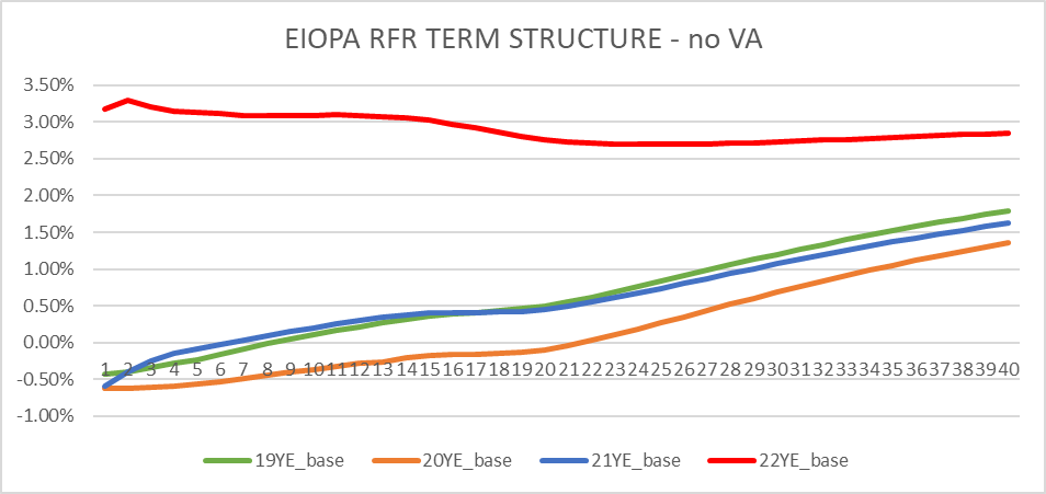
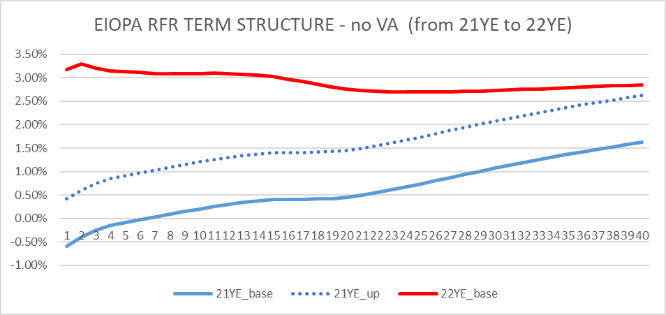
The following chart shows the evolution of the RFR published by EIOPA in the past four years: the economic scenario has completely changed from a “low lasting yield” perspective to a baseline where there are no signs rates will be dropping any time soon. From 21YE to 22YE a 300-bps rise has been experienced in the very short term, turning into a term structure that is no more increasing monotone and looks almost flat.
Less than two weeks ago, both the European Central Bank (ECB) and the United States Federal Reserve (FED) raised again the interest rates, reaching benchmarks of respectively 3.25% and 5.25%, the highest levels registered since November 2008 and August 2007. These were respectively the seventh and eighth consecutive rate rises carried out by the two institutions. The ECB indicated its intent to continue the hikes going forward, while the FED hinted this could be the last in its own historic series. Both decisions were taken to tackle the inflation and bring it down to a moderate level. The ECB’s one came after an increase to 7% of the headline inflation rate registered in April and the estimates published by the International Monetary Fund (IMF) suggesting a core inflation (that excludes food and energy prices) not reaching the ECB target (2%) until 2025, albeit its recent slight decrease to 5.6% in April. Even though higher interest rates help to curb soaring prices, they can also take a toll in the real economy, increasing the borrowing cost: indeed, a recent ECB survey showed that the banks have tightened access to credit, with the biggest drop in demand for loans registered over a decade. This trend could set a domino effect, dragging further on economy growth, that has barely moved during the last quarter.
Besides that, when rates increase, the market values of Assets decrease, boosting the unrealized losses of banks and life insurance companies holding the financial securities. Apart from the challenges coming from the regulatory capital absorption, this situation becomes a true issue when the customers withdraw their money, whether in a form of cash deposit or policy, forcing the institution to sell the Assets and turn the losses from theorical (unrealized) to actual (realized); the true issue becomes a big problem when it goes in hand with the lack of liquidity.
The financial market has recently attended three of these examples: the default of the Silicon Valley bank in mid-March, the rescue of Credit Swiss by its competitor UBS and the acquisition of First Republic by JP Morgan. In all the three cases, the bankruptcy risk, and the fear of losing their savings, encouraged the clients to leave, triggering a self-fulfilling prophecy.
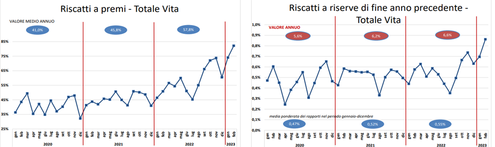
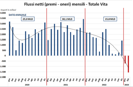
On the life insurances side, the statistics recently published by ANIA (references [1] and [2]), the National Associations of Italian Insurers, showed a significant increase in lapses (lapse rate from 5.5% in 2020 to 6.7% in 2022), with a boost registered in the last quarter of 2022, that continued in the first months of 2023, turning into negative net flows (premiums minus benefits) for the life insurance companies. In 2022 the total outflows were around 78.5 billion, 70% of which attributable to lapses. Out of these 54.5 billion, 17 were registered in the last quarter (+12.5% compared to 2021) and in February 2023, the lapses reached a peak of 7 billion, with an annual increase around 47%. The saving and investment insurance policies seem no longer able to compete with the high yields provided by BTPs or other deposit accounts.
As said, the SII Directive aims at minimizing the risk for the policyholders to incur a loss in case of failure of the insurance institutions: the SR shall be higher than 100%, and the higher the better. The directive requires a calculation of the BEL that embeds the likelihood of policyholders to exercise contractual options, including lapses and surrenders, supposing a rational conduct in accordance with the market movements, and requires to hold a SCR to cover several risks, among which the rise or fall of the interest rates (IR risk) and the withdrawal of money by the policyholder (Lapse risk).
In a context of high rates, a rationale policyholder is expected to surrender its saving or unit linked insurance policy to buy an alternative instrument that provides a higher yield. The modelling of the Dynamic Policyholder Behavior (DPHB) is particularly relevant in stochastic scenarios, where the dynamic lapses are path dependent. The regulation does not provide a specified formula, but hints some guidelines to follow, such as the need of the risk to be bidirectional and the need of considering the interaction between the DPHB and the Future Management Actions (FMA), that directly influence the contract return, to compare to the market one. The directive also requires all the relevant contractual options to be considered and the exercise rate to be set on both statistical evidence and a sound Expert Judgement, clarifying that the lack of data in extreme scenario does not prevent from assuming the option to be exercised. If the DPHB modelling works properly, in a situation of profitable business and increasing interest rates, the OF drop because of the increase in TP lead by the higher cost of exercise of the options embedded in the contract.
Under the SF, the IR risk capital requirement is defined as the larger of the following:
The interest rate risk sub-module flows into market risk module with a correlation to the Equity, Property and Spread risks that varies according to the biting scenario, with the interest up being the most diversified. The exposure to the IR risk follows the Asset/Liabilities duration gap: positive gaps (Assets longer than Liabilities) suffer an increase in interest rates, negative gaps suffer a decrease in interest rates. Life insurance companies tend to adjust their Assets duration to match the liabilities one, therefore avoiding a significant interest rate risk capital absorption. Usually, the business model of life insurance companies is long termed, being their liabilities characterized by quite high durations, and the duration gap slightly negative, but this can vary from undertaking to undertaking and, within the same undertaking, from segregated fund to segregated fund. In a context of increasing rates, the discount effect on the liability side is stronger than on the Asset side, resulting in a gain/loss of OF for negative/positive durations gaps, accompanied by an increase in the SCR IR risk module, that comes from the nature of the stress: a relative shock gets bigger in absolute terms when applied to a higher base. However, the IR risk magnitude can be kept under control by matching the durations, while the lapse risk remains challenging in context of high rates. Indeed, in this scenario, policyholders are expected to lapse more, and profitable businesses suffer from both a decrease in OF and an increase in SCR, with a significant impact in the lapse risk module, driven by the mass scenario. Indeed, the lapse risk capital requirement measures the adverse changes in liabilities due to a change in expected exercise rates and is defined as the larger of the following:
As discussed in the following, the SF appears to underestimate the IR risk (both in case of downward and upward movement), and to overestimate the lapse mass risk. To make up for the former issue, with the goal of ensuring a better protection to the policyholders, in September 2021 the European Commission (EC) published a legislative package aimed at amending the SII Directive. The latter issue, instead, has been investigated by the market, where life insurance companies adopting the SF looked for different solutions aimed at mitigating the massive increase in the SCR driven by the lapse mass scenario in a context of high rates.
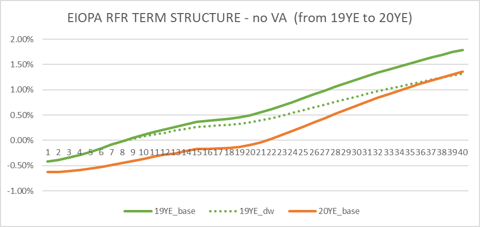
Albeit everybody knows how hard is to predict the future rate environment, the following charts show that the EIOPA expectations of a rate decrease / increase (as a stress at a 99.50% confidence level over a 1-year period) have proved not to be adequate compared to the actual 1-year movement registered back in December 2019 (19YE_dw vs 20YE_base) and December 2021 (21YE_up vs 22YE_base). The areas between the green/blue dotted line and the orange/red one indicate the underestimation of the downward/upward risk by the SF, with the actual movement over one year much larger compared to the one expected to happen one every 200 years.
To fix this issue, the EC hinted to modify the IR risk calibration into a relative shift approach, with a phase-in mechanism of 5 years. The details of the calculation will be released in an update of the Delegates Acts, likely following the proposal from EIOPA, with shocked interest rates in the downward scenario floored to a minimum of -1.25%. The legislative proposal published by the EC is now being discussed by Member States, Stakeholders, and the European Parliament (EP), and the finalization of the legislative process may last few years.
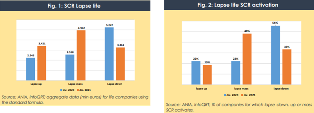
Concerning the capital requirement needed to cover the lapse risk, the nature of the shock envisaged by the SF for the mass scenario (40% of immediate redemptions) seems to be unrealistic, also when compared to the stress level indicated by EIOPA in the 2021 Stress Test (20% of immediate redemptions) which is also like the average shock calibrated by the companies adopting the internal model. Furthermore, it can be questioned the good sense of maintaining the same base lapse assumptions and DPHB rules after this kind of shock: probably, it would be more realistic to decrease the base lapse level. As shown in the following bar diagrams (Fig 1 and Fig 2, reference #[3]), together with the increase in the interest rates and the DPHB application, the lapse mass scenario has significant hit the SII position of undertakings using the SF, where the lapse mass risk has doubled in terms of aggregate SCR, becoming the predominant lapse scenario among the three.
In its July 22 report on the SII trends [3], ANIA pointed out that the current methodology of the SF presents dome critical elements, including assumptions and parameters inconsistent with the real Dynamics of the PHB; it also hinted the adoption of specifical reinsurance contracts to be too little, although, back in July 2021, EIOPA recommended to consider similar solutions in its “Opinion on the use of risk mitigating techniques by insurance and reinsurance undertakings”. To mitigate these issues, life insurance companies started looking for different solutions aimed at increasing the SR, both reducing the SCR or increasing the OF. Based on the public information as at 22YE, different undertakings have already implemented mass lapse reinsurance treaties. An example of mass lapse treaty is provided in the following.
A mass lapse reinsurance treaty is a stop-loss cover against the lapse mass risks, that limits the losses in OF in a range defined by:
The following chart shows an illustrative reinsurance structure with an attachment and detachment points corresponding to a lapse rate of respectively 20% and 40%.
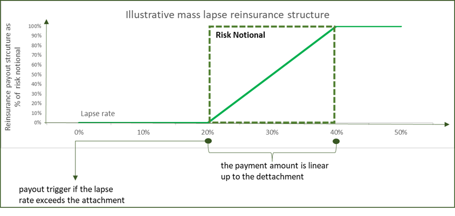
The resulting payout follows the potential losses in OF faced by the undertaking between the attachment and detachment points and grows linearly: no reimbursements are due before the attachment point and no further reimbursements are due after the detachment point. The maximum payout payable by the reinsurer, generally referred to as the “Risk Notional”, dotted line area in the chart, represents the difference in OF losses measured in the detachment and attachment points and is used to derive the reinsurance premium. The reinsurance premium is indeed represented by a fee of the Risk Notional and is set by the reinsurer based on a number of factors, such as the company’s best estimate lapse rates, the type of business, the distribution channels, and the level of risk transfer to achieve (the lower the attachment lapse rate, the higher risk transfer). The duration of the reinsurance cover is set upon request and is usually higher than 2 years, to allow for the Solvency II eligibility, where the SCR is defined over a 1-year horizon.
Beside the reduction in the exposure to potential actual mass lapse events, the key impacts on the SR are driven by the reduction in:
References:

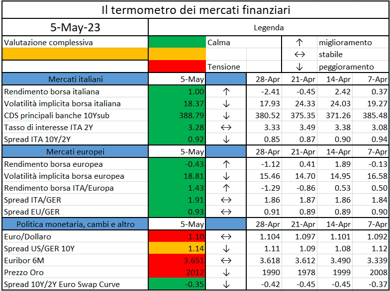
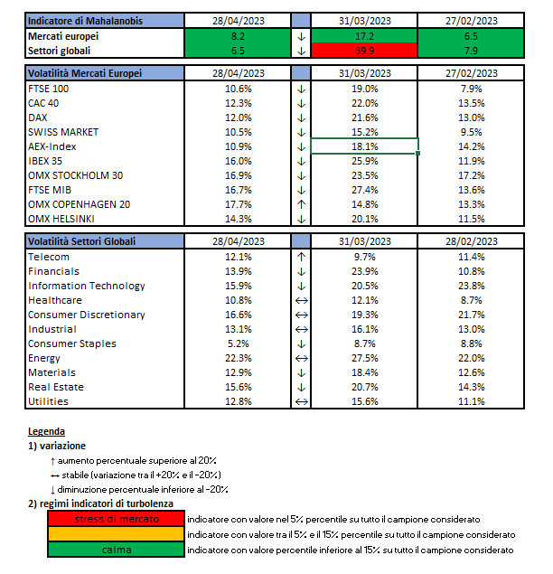
L’iniziativa di Finriskalert.it “Il termometro dei mercati finanziari” vuole presentare un indicatore settimanale sul grado di turbolenza/tensione dei mercati finanziari, con particolare attenzione all’Italia.
Significato degli indicatori
I colori sono assegnati in un’ottica VaR: se il valore riportato è superiore (inferiore) al quantile al 15%, il colore utilizzato è l’arancione. Se il valore riportato è superiore (inferiore) al quantile al 5% il colore utilizzato è il rosso. La banda (verso l’alto o verso il basso) viene selezionata, a seconda dell’indicatore, nella direzione dell’instabilità del mercato. I quantili vengono ricostruiti prendendo la serie storica di un anno di osservazioni: ad esempio, un valore in una casella rossa significa che appartiene al 5% dei valori meno positivi riscontrati nell’ultimo anno. Per le prime tre voci della sezione “Politica Monetaria”, le bande per definire il colore sono simmetriche (valori in positivo e in negativo). I dati riportati provengono dal database Thomson Reuters. Infine, la tendenza mostra la dinamica in atto e viene rappresentata dalle frecce: ↑,↓, ↔ indicano rispettivamente miglioramento, peggioramento, stabilità rispetto alla rilevazione precedente.
Disclaimer: Le informazioni contenute in questa pagina sono esclusivamente a scopo informativo e per uso personale. Le informazioni possono essere modificate da finriskalert.it in qualsiasi momento e senza preavviso. Finriskalert.it non può fornire alcuna garanzia in merito all’affidabilità, completezza, esattezza ed attualità dei dati riportati e, pertanto, non assume alcuna responsabilità per qualsiasi danno legato all’uso, proprio o improprio delle informazioni contenute in questa pagina. I contenuti presenti in questa pagina non devono in alcun modo essere intesi come consigli finanziari, economici, giuridici, fiscali o di altra natura e nessuna decisione d’investimento o qualsiasi altra decisione.
L’attuale disciplina della gestione delle crisi bancarie lascia aperti dubbi interpretativi, non ancora chiariti dalla giurisprudenza europea. D’altra parte, accanto al confronto costante in sede europea, si avverte la necessità di approfondire…
The paper presents the general features of the Risk Dashboard as an instrument for macroprudential supervision of the financial sector and motivates why it could also be useful in monitoring the specific risks
of insurance…
https://www.ivass.it/pubblicazioni-e-statistiche/pubblicazioni/quaderni/2023/iv26/Quaderno_26.pdf
The inflation outlook continues to be too high for too long. In light of the ongoing high inflation pressures, the Governing Council today decided to raise the three key ECB interest rates by 25 basis points…
https://www.ecb.europa.eu//press/pr/date/2023/html/ecb.mp230504~cdfd11a697.en.html

Il binomio Bitcoin-blockchain è oramai divenuto molto popolare, andando oltre il mondo degli addetti ai lavori, cioè degli esperti di tecnologia e di finanza.
Bitcoin ha attratto molti per il suo mirabolante andamento: a partire dal 2015, in poco più di sei anni, il prezzo dei Bitcoin è aumentato di duecento volte salvo poi scendere a meno della metà del picco a fine 2022. Oggi circa il 2,2% delle famiglie italiane detengono criptovalute: può sembrare poco, ma in realtà è molto se si pensa che le famiglie che detengono direttamente titoli azionari sono meno dell’8%.
La Blockchain ha suscitato interesse per il suo nome esotico, pochi però sanno davvero come funziona. Inoltre il binomio Blockchain-Bitcoin è spesso salito agli onori della cronaca per i traffici illeciti, o per i riscatti di attacchi cyber, ma non c’è solo questo. È infatti portatore di novità importanti che potrebbero impattare la nostra vita in un prossimo futuro.
Per questo HuffingtonPost e il QFinLab, il laboratorio di finanza quantitativa del Dipartimento di Matematica del Politecnico di Milano, hanno pensato ad un percorso di video nel quale entrare nel merito, con termini semplici, a costo di non essere precisi al 100%, sugli aspetti tecnici. Con il desiderio di farvi capire gli aspetti tecnologici, quali sono i vantaggi, le potenzialità e i rischi di questa nuova tecnologia.
Non ci resta che augurarvi… una buona visione!
https://www.huffingtonpost.it/dossier/criptovalute-in-parole-semplici

L’indicatore di Mahalanobis permette di evidenziare periodi di stress nei mercati finanziari. Si tratta di un indicatore che dipende dalle volatilità e dalle correlazioni di un particolare universo investimenti preso ad esame. Nello specifico ci siamo occupati dei mercati azionari europei e dei settori azionari globali.
Gli indici utilizzati sono:

Le volatilità riportate sono storiche e calcolate sugli ultimi 30 trading days disponibili. Per ogni asset-class dunque sono prima calcolati i rendimenti logaritmici dei prezzi degli indici di riferimento, successivamente si procede col calcolo della deviazione standard dei rendimenti, ed infine si procede a moltiplicare la deviazione standard per il fattore di annualizzazione.
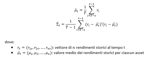
Per il calcolo della distanza di Mahalnobis si procede dapprima con la stima della matrice di covarianza tra le asset-class. Si considera l’approccio delle finestre mobili. Come con la volatilità, si procede prima con il calcolo dei rendimenti logaritmici e poi con la stima storica della matrice di covarianza, come riportato di seguito.
Supponendo una finestra mobile di T periodi, viene calcolato il valore medio e la matrice varianza covarianza al tempo t come segue:
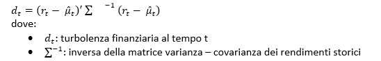
La distanza di Mahalanobis è definita formalmente come:
Le parametrizzazioni che sono state scelte sono:
Le statistiche percentili sono state calcolate a partire dalla distribuzione dell’indicatore di Mahalanobis dal Dicembre 1997 al Dicembre 2019 su rilevazioni mensili.
Ulteriori dettagli sono riportati in questo articolo.
Disclaimer: Le informazioni contenute in questa pagina sono esclusivamente a scopo informativo e per uso personale. Le informazioni possono essere modificate da finriskalert.it in qualsiasi momento e senza preavviso. Finriskalert.it non può fornire alcuna garanzia in merito all’affidabilità, completezza, esattezza ed attualità dei dati riportati e, pertanto, non assume alcuna responsabilità per qualsiasi danno legato all’uso, proprio o improprio delle informazioni contenute in questa pagina. I contenuti presenti in questa pagina non devono in alcun modo essere intesi come consigli finanziari, economici, giuridici, fiscali o di altra natura e nessuna decisione d’investim
L’attività economica globale è rallentata nel periodo estivo e le stime di crescita nelle principali economie sono state riviste al ribasso per il prossimo anno. Il ciclo economico mondiale rimane fortemente condizionato dall’elevata inflazione, dalle difficoltà di approvvigionamento energetico e alimentare causate dal protrarsi del conflitto in Ucraina e acuite dalla siccità, nonché dal rallentamento dell’economia cinese…
https://www.bancaditalia.it/media/notizia/rapporto-sulla-stabilit-finanziaria-n-1-2023/
